|
|
|
|
Subsalt imaging by target-oriented wavefield least-squares migration: A 3-D field-data example |
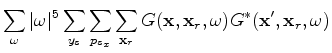
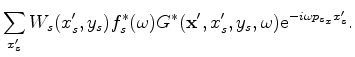
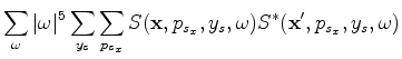
As derived in Appendix A, each component of the the 3-D conical-wave domain Hessian reads
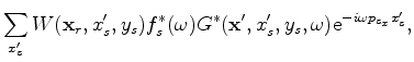 is the source signature at frequency
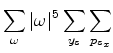
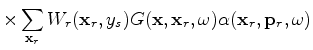
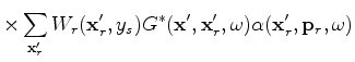
The diagonal part of the Hessian (when
![]() ), which contains autocorrelations
of both source and receiver-side Green's functions, can be interpreted as a subsurface illumination
map with contributions from both sources and receivers. The rows of the Hessian (for fixed
), which contains autocorrelations
of both source and receiver-side Green's functions, can be interpreted as a subsurface illumination
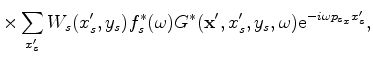
map with contributions from both sources and receivers. The rows of the Hessian (for fixed ![]() 's
and varying
's
and varying ![]() ), which contains crosscorrelations of both source and receiver-side Green's
functions, can be interpreted as resolution functions (Tang, 2009; Lecomte, 2008). They measure
how much smearing an image can have due to a given acquisition setup.
), which contains crosscorrelations of both source and receiver-side Green's
functions, can be interpreted as resolution functions (Tang, 2009; Lecomte, 2008). They measure
how much smearing an image can have due to a given acquisition setup.
The exact Hessian defined by equation 3, however, is nontrivial and very expensive to implement.
It requires either storing a huge number of Green's functions for reuse, or performing
a large number of wavefield propagations to repeatedly calculate the Green's functions, resulting in
a computational cost proportional to
![]() , with
, with
![]() ,
, ![]() ,
, ![]() and
and ![]() being the number of crossline shots,
inline conical waves, inline receivers and crossline receivers, respectively.
being the number of crossline shots,
inline conical waves, inline receivers and crossline receivers, respectively.
In order to reduce the computational cost,
we use the simultaneous phase-encoding technique to efficiently
calculate an approximate version of equation 3.
The simultaneous phase-encoding, however, is only strictly valid when the
acquisition
mask operator is independent along the encoding axes (Tang, 2009).
For the 3-D conical-wave-domain Hessian, the encoding axes are the inline source axis ![]() and the
receiver axis
and the
receiver axis
![]() , respectively.
Ocean-bottom cable (OBC) and land acquisition geometries, where receivers are fixed for all sources, obviously
satisfy this condition. But marine-streamer acquisition geometry, where the receiver cable moves with sources,
apparently does not.
To make the theory applicable to the marine-streamer data case,
we assume that the receiver location
, respectively.
Ocean-bottom cable (OBC) and land acquisition geometries, where receivers are fixed for all sources, obviously
satisfy this condition. But marine-streamer acquisition geometry, where the receiver cable moves with sources,
apparently does not.
To make the theory applicable to the marine-streamer data case,
we assume that the receiver location ![]() depends only on the crossline source position
depends only on the crossline source position ![]() ,
but is independent of the inline source position
,
but is independent of the inline source position ![]() .
This implicitly assumes that for a fixed crossline
.
This implicitly assumes that for a fixed crossline ![]() , all inline shots share the same receiver array.
Therefore, we can express the acquisition mask operator as a product of two separate functions:
, all inline shots share the same receiver array.
Therefore, we can express the acquisition mask operator as a product of two separate functions:
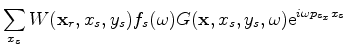
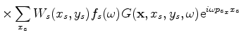
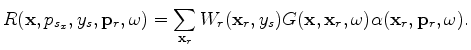
Substituting equation 4 into equation 3 yields
 is the receiver-side encoding function, to be specified later.
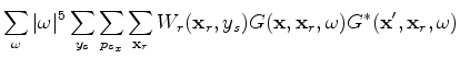
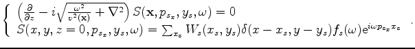
Equation 6 can be greatly simplified as follows:
is the receiver-side encoding function, to be specified later.
Equation 6 can be greatly simplified as follows:
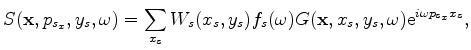
 and
and 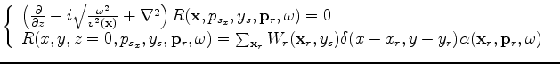 is the velocity at image point is the wavefield generated by propagating the conical-wave source
However, the phase-encoded Hessian brings unwanted crosstalk. This becomes clear by comparing equations 6
and 3. The crosstalk can be suppressed by carefully choosing the phase-encoding function (Tang, 2009).
In this paper, we choose to be a random phase-encoding function; thus ![]() denotes the realization index of the random phase-encoding function.
It would be very easy to verify that, with this choice of encoding functions, the expectation of the crosstalk becomes zero.
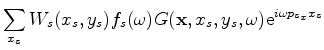
Therefore,
equation 6 converges
to equation 5 by stacking over
denotes the realization index of the random phase-encoding function.
It would be very easy to verify that, with this choice of encoding functions, the expectation of the crosstalk becomes zero.
Therefore,
equation 6 converges
to equation 5 by stacking over ![]() , according to the law of large numbers (Gray and Davisson, 2003):
, according to the law of large numbers (Gray and Davisson, 2003):
| (12) |
|
|
|
|
Subsalt imaging by target-oriented wavefield least-squares migration: A 3-D field-data example |