Subsalt imaging by target-oriented wavefield least-squares migration: A 3-D field-data example

Regularizations

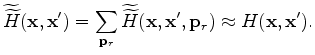
Regularization helps to stabilize the inversion; it can shape the null space and remove unwanted features in the inverted result by introducing user-defined model-covariance operators. In this paper, we choose to use the following regularization term:

$${\mathcal R}({\bf m}) = \frac{1}{2}\vert\vert{\bf D}^{*}{\bf D}{\bf m}\vert\vert^2,$$ (13)

where operator 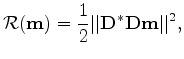${\bf D}$ contains wavekill filters (Claerbout, 2008), which annihilate local planar-events with given dips. The operator imposes continuity of reflectors along its dipping direction. This idea has also been explored by Clapp (2005) and Ayeni et al. (2009), who use similar filters (Hale, 2007; Clapp, 2003) to regularize the data-domain least-squares migration.

Instead of solving the inversion problem as a regularization problem, we solve it as a preconditioning problem by making change of variables as follows:

$${\bf m} = {\bf S}{\bf n},$$ (14)

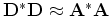
where ${\bf n}$ is the vector of preconditioned variables and ${\bf S}$ is the preconditioning operator, which is defined to be an approximate inverse of the regularization operator ${\bf D}^{*}{\bf D}$. To find the inverse of ${\bf D}^{*}{\bf D}$, we factorize it into minimum-phase filters ${\bf A}$ such that ${\bf D}^{*}{\bf D}\approx{\bf A}^{*}{\bf A}$. We use the Wilson-Burg factorization (Fomel et al., 2003; Claerbout, 1992) and apply it on the helix (Claerbout, 2008,1998). Since minimum-phase filters have stable inverses, we can define the preconditioning operator as follows:

$${\bf S} = {\bf A}^{-1}\left({\bf A}^{*}\right)^{-1}.$$ (15)

Unlike ${\bf D}^{*}{\bf D}$, operator ${\bf S}$ contains dip filters, which smooth along given dip directions. Substituting equations 13, 14 and 15 into 1 yields

$$J_{p}({\bf n}) = \frac{1}{2}\vert\vert{\bf H}{\bf S}{\bf n}-{\bf m}_{\rm mig}\vert\vert^2 + \epsilon \vert\vert{\bf n}\vert\vert^2.$$ (16)

Objective function 16 is often solved by setting $\epsilon=0$ and iterating until an acceptable result is obtained (Claerbout, 2008). Solving it in this way implicitly assumes that we are starting with a model that has all the user-defined covariance, and that the more iterations we run, the more we honor the data. Once a solution vector ${\bf n}_{\rm sol}$ has been found, the final model is obtained by computing ${\bf m}_{\rm sol} = {\bf S}{\bf n}_{\rm sol}$.

Subsalt imaging by target-oriented wavefield least-squares migration: A 3-D field-data example