|
|
|
|
Subsalt velocity analysis by target-oriented wavefield tomography: A 3-D field-data example |
We use the normalized DSO (equation 5) to optimize the subsalt velocity.
Although the 3-D Born data set is synthesized with both inline and crossline subsurface offsets, we
use only inline subsurface offsets for velocity inversion due to the limited angular coverage in the crossline direction.
We regularize the inversion by smoothing the gradient using a B-spline operator as follows:
| (6) |
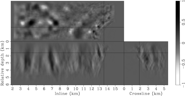
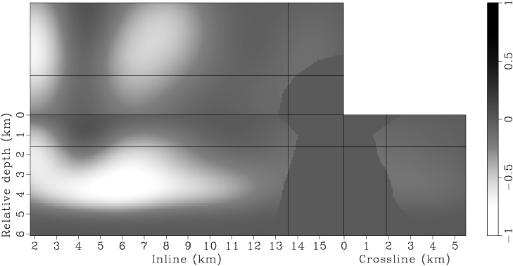
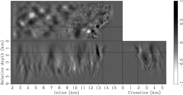
Instead of using a fixed degree for gradient smoothing, we gradually decrease the smoothness of the gradient after every few iterations by decreasing the spacing of the B-spline nodes. We have found this strategy effective in finding an acceptable minimum, even when starting with a velocity model far from being accurate. Decreasing the smoothness of the gradient at later iterations also helps improve the resolution of the velocity model. This procedure is similar to the multi-scale inversion strategy, which has proven useful in practice (Bunks et al., 1995; Soubaras and Gratacos, 2007). Table 1 illustrates the spacings of the B-spline nodes for different iterations. Figures 7 presents the raw and smoothed gradients at different iterations.
| Iterations | Node spacing in |
Node spacing in |
Node spacing in |
|
|---|
|
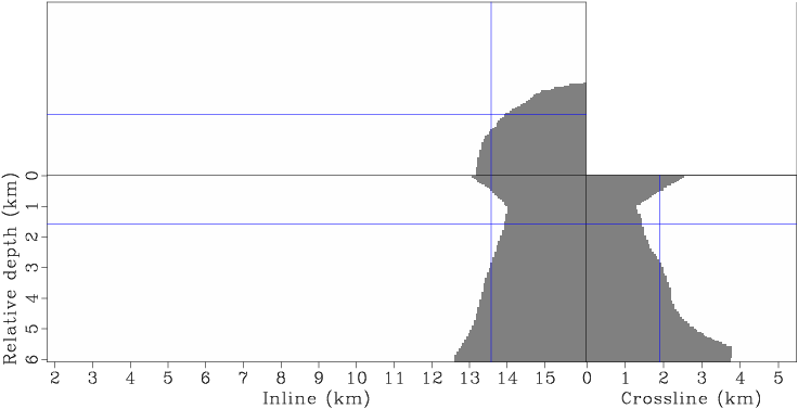
bpgom3d-gmsk-target
Figure 6. The mask operator applied to the gradient to prevent updating the velocity inside the salt. [CR] |
|
|
|
|---|
|
r1,s1,r11,s11,r21,s21,r31,s31
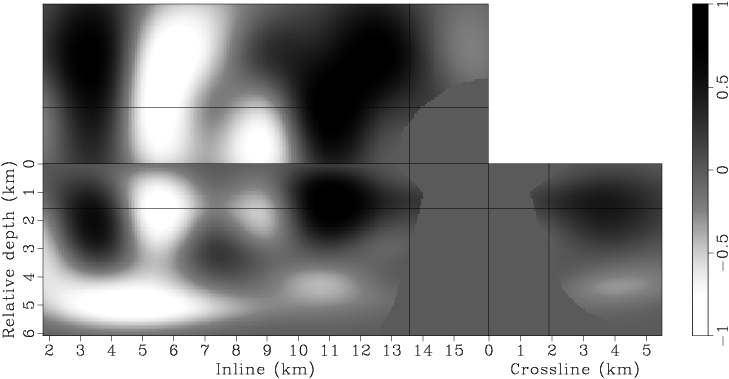
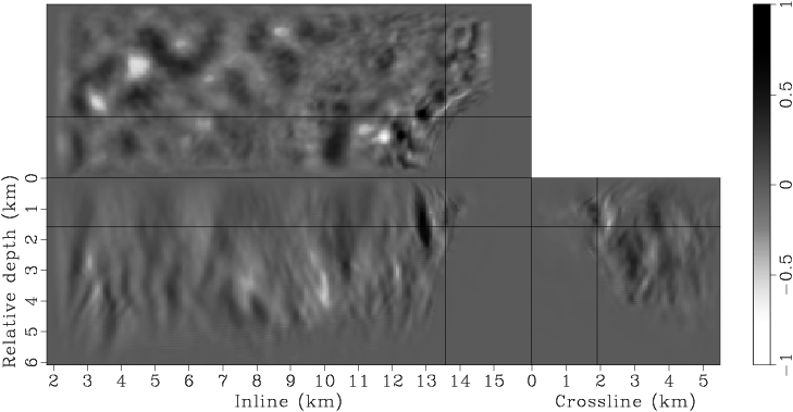
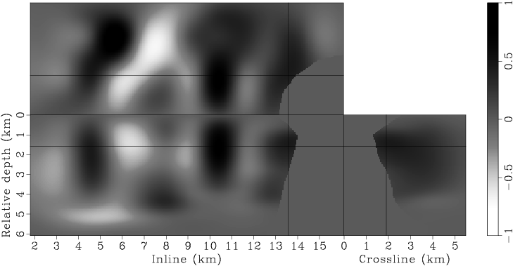
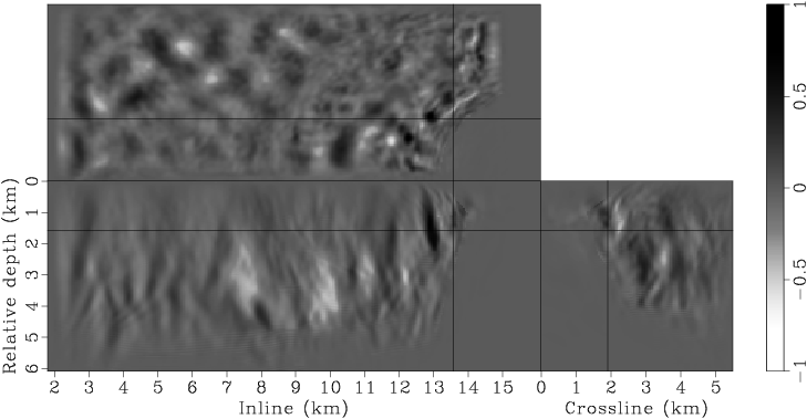
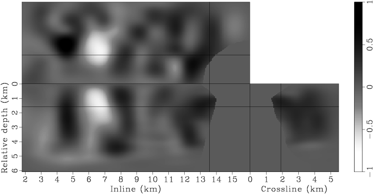
Figure 7. Panels (a), (c), (e), (g) are the raw gradients at iterations |
|
|
We restart the nonlinear conjugate gradient solver every ![]() iterations, and
we terminate the inversion after
iterations, and
we terminate the inversion after ![]() iterations when the objective function does not decrease significantly.
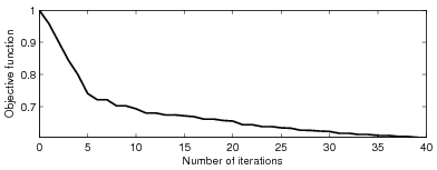
Figure 8 shows
how the objective function evolves over the first
iterations when the objective function does not decrease significantly.
Figure 8 shows
how the objective function evolves over the first ![]() iterations,
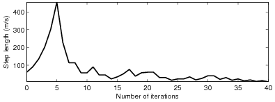
whereas Figure 9 plots the step lengths as a function of iterations. It seems
that the objective function converges very fast at the first several iterations, then
the convergence slows down quickly, and that the velocity model gets the most significant updates
at the first several iterations.
iterations,
whereas Figure 9 plots the step lengths as a function of iterations. It seems
that the objective function converges very fast at the first several iterations, then
the convergence slows down quickly, and that the velocity model gets the most significant updates
at the first several iterations.
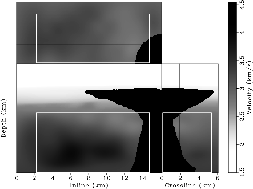
The final velocity model obtained by merging the inverted velocity model in the target region with the velocity model above the target is shown in Figure 10. It is interesting to note that the velocities beneath the salt body are slightly lower than the surrounding sediment velocities. The low velocities might indicate overpressure due to the compaction of the salt body.
|
|---|
|
fobj
Figure 8. The evolution of the objective function over the first |
|
|
|
|---|
|
step
Figure 9. Step length versus the number of iterations. The initial step length is about |
|
|
|
|---|
|
bpgom3d-vmod-full
Figure 10. The final velocity model after merging the inverted velocity model in the target region with the velocity model above the target. [CR] |
|
|
|
|
|
|
Subsalt velocity analysis by target-oriented wavefield tomography: A 3-D field-data example |