Random boundary condition for low-frequency wave propagation

Low-frequency modeling

Figure 2 and 3 shows wavefields at 3.5 seconds using a point source with a peak frequency of $6$ Hz in velocity fields with the different boundary regions mentioned in Figure 1. The top row of figure 2 shows 2D slices of the wavefield using one realization of each velocity. For a $6$ Hz peak frequency (which is typical in waveform inversion), a random boundary with small grain size is only slightly better than constant velocity. In this case, the dominant wavelength is $500$ m, and only when grain size becomes comparable to the dominant wavelength does the wavefield start to appear random. However, there are some low-frequency residuals remaining in the images using big cubic grains. The bottom row of figure 2 shows a stacked wavefield of the same source and record time using $16$ different realizations of random boundaries. It is now obvious that the low-frequency residuals are evidence of poor performance from using big cubic grains. The regular shape of these cubic grains cannot scatter certain incident wavefronts, thus leaving coherent energy at these angles. Randomly shaped grains, on the other hand, scatter those low-frequency components quite well. This can be seen in the wavenumber domain amplitude spectrum of these wavefields (Figure 3), where the randomly shaped grains reduce lower-wavenumber components much more effectively than cubic grains.

wvmvsixhoriz
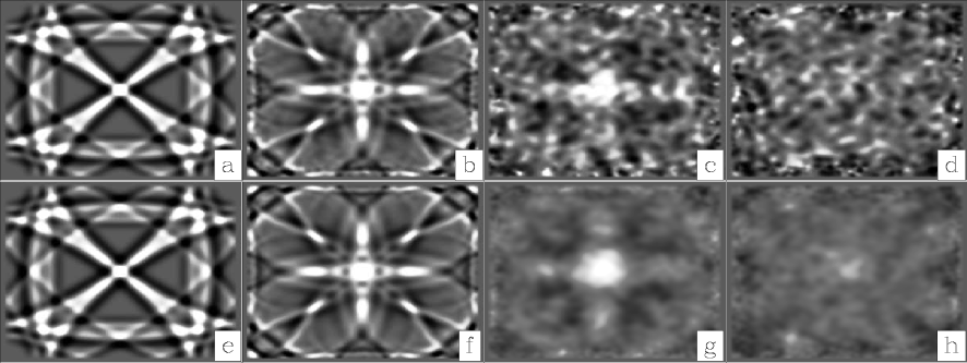
Figure 2. Time-domain wavefield snapshots for a point source with $6$ Hz peak frequency in velocity fields with different random boundary conditions. The top row shows one realization of velocity with a) constant velocity, b) cubic grains with $20$ m side length, c) cubic grains with $200$ m side length, and d) randomly shaped grains with effective length $200$ m. The bottom row shows average wavefields using $16$ realizations of velocity with e) constant velocity, f) cubic grains with $20$ m side length, g) cubic grains with $200$ m side length, and h) randomly shaped grains with $200$ m effective length. [CR]

wvmvsixkabshoriz
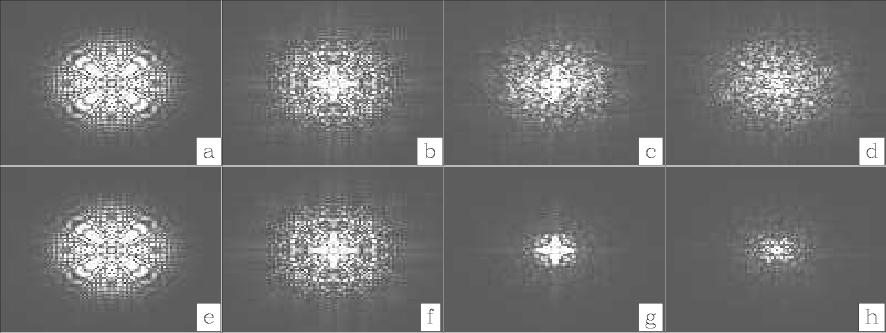
Figure 3. Wave-number-domain amplitude spectrum of wavefield snapshots for a point source with $6$ Hz peak frequency in velocity fields with different random boundary conditions. The top row shows one realization of velocity with a) constant velocity, b) cubic grains with $20$ m side length, c) cubic grains with $200$ m side length, and d) randomly shaped grains with effective length $200$ m. The bottom row shows average wavefields using $16$ realizations of velocity with e) constant velocity, f) cubic grains with $20$ m side length, g) cubic grains with $200$ m side length, and h) randomly shaped grains with $200$ m effective length. [CR]

Random boundary condition for low-frequency wave propagation