Random boundary condition for low-frequency wave propagation

Examples

velview
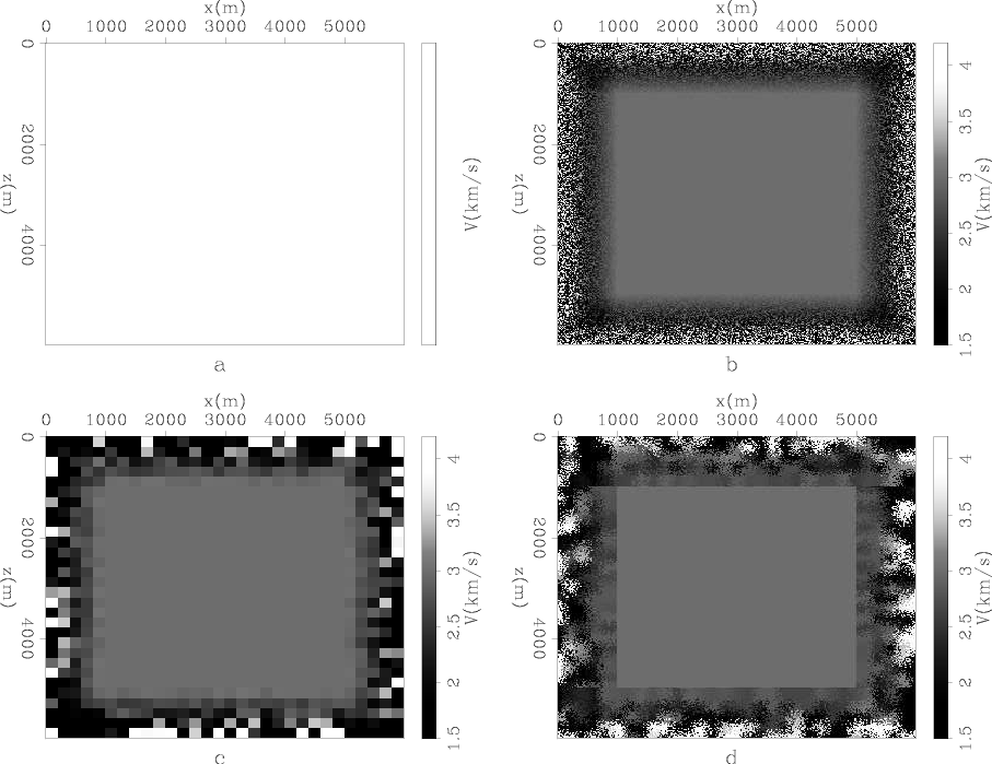
Figure 1. Velocity with different boundary regions: a) constant velocity ; b) cubic grains with $20$ m side length ; c) cubic grains with $200$ m side length; d) randomly shaped grains with $200$ m effective length. [ER]

To illustrate the idea, we show examples of acoustic modeling using constant velocity fields with random boundaries of different ``grain'' size and shape. Each example is compared with a constant boundary condition, where wavefields propagate through boundary regions that have the same velocity values as the inner region. In addition, we use zero-value boundary conditions when wavefields reach the end of each boundary region. The entire velocity field, including the boundary regions, is $6000$ meters in $x$ ,$y$ and $z$ , with the same $20$ -meter spacing used in all directions. Boundary regions are $1000$ meters ($50$ gridpoints) in each direction, and either the velocity is constant throughout the region, or velocity values are randomly assigned different grain sizes. In the inner region of the velocity fields, the velocity is constant at $3$ km/s; in the boundary regions the velocity is at least 1.5 km/s and no greater than $4.2$ km/s. Two types of grains are used in random boundaries, shown in Figure 1: cubic grains with two different side lengths: $20$ m ($1$ grid point )and $200$ m ($10$ grid point), and randomly shaped grains with effective length of $200$ m ($10$ grid points). 3-D modeling is used for all examples, but for display purposes, we only show 2D slices of 3D velocity and wavefields.

Random boundary condition for low-frequency wave propagation