|
|
|
|
Least-squares reverse time migration for the Cascadia ocean-bottom dataset |
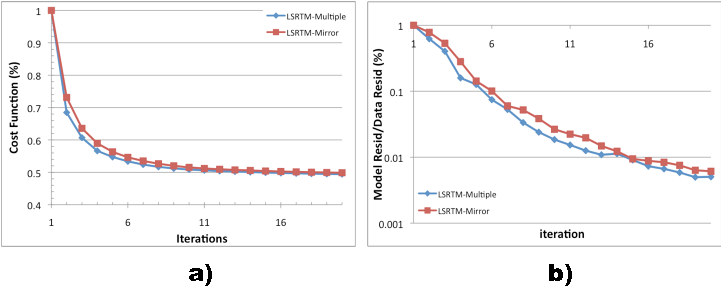
We use the iterative conjugate direction method to minimize our objective function.
Figure 8 (a) shows the value of the objective function over 20 iterations.
The inversion converges nicely with the residuals dropping to 50![]() of the original value.
It is important to point out that the final residual drops is problem dependent.
In general, if the raw dataset contains a low signal-to-noise ratio, then the residual drop will be less.
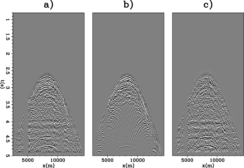
Figure 9 (a) shows a common receiver gather for this data set. After 20 iterations, the corresponding forward modeled data 9 (b) is able to capture most of the prominent signal in the data. The difference of the two yields the data residual shown in Figure 9 (c).
of the original value.
It is important to point out that the final residual drops is problem dependent.
In general, if the raw dataset contains a low signal-to-noise ratio, then the residual drop will be less.
Figure 9 (a) shows a common receiver gather for this data set. After 20 iterations, the corresponding forward modeled data 9 (b) is able to capture most of the prominent signal in the data. The difference of the two yields the data residual shown in Figure 9 (c).
Another way to evaluate convergence is to study the ratio of the model residual over data residual. The model residual is defined to be applying the migration operator to the data residual at each iteration. (It is also called the gradient.) In Figure 8 (b), we can see that the ratio almost drops down to zero over iterations, which also indicates convergence.
|
|---|
|
ResidualPlot
Figure 8. (a) Objective function over 20 iterations and (b) The ratio of model residual over data residual over 20 iterations (Note in log scale). |
|
|
|
|---|
|
DatspaceResid
Figure 9. (a) A common receiver gather after pre-prosessing for one of the ocean-bottom seismometer, (b) the forward modeled data of the same gather using the LSRTM-M reflectivity image at the 20th iteration and(c) the data residual of the same gather at the 20th iteration, which is equivalent to the difference between (a) and (b). |
|
|
|
|
|
|
Least-squares reverse time migration for the Cascadia ocean-bottom dataset |