|
|
|
|
Least-squares reverse time migration for the Cascadia ocean-bottom dataset |
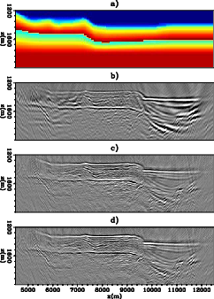
Figure 6 (b) shows the mirror-imaging RTM result. Overall, we can identify some migration artifacts associated with RTM, such as the high-amplitude low-frequency artifacts. The resolution is low, and the structural information below the BSR is generally difficult to identify.
|
|---|
|
RTMinv
Figure 6. (a) Migration velocity model, (b) RTM image of the mirror signal, (c) LSRTM of the mirror signal (LSRTM-M), and (d) LSRTM of mirror and higher-order mirror signals (LSRTM-HM). |
|
|
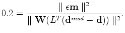
Seismic inversion is an ill-posed problem.
To prevent divergence to unrealistic solutions, we add an additional term to our objective function
![]() .
In Ronen and Liner (2000); Nemeth et al. (1999), data weighting operators are used to remove the acquisition footprint by having zero weighting on regions corresponding to the acquisition gap.
The overall fitting goal becomes
.
In Ronen and Liner (2000); Nemeth et al. (1999), data weighting operators are used to remove the acquisition footprint by having zero weighting on regions corresponding to the acquisition gap.
The overall fitting goal becomes
| (4) |
| (5) |
 of the gradient contribution from the data fitting term.
From experiments with both synthetic and field dataset, we found that this limit yields satifactory results.
For this dataset, the damping term alone seems to adequately regularize the inversion and yield a satisfactory result.
For more complex survey regions, other regularization terms are needed to further constrain the inversion.
of the gradient contribution from the data fitting term.
From experiments with both synthetic and field dataset, we found that this limit yields satifactory results.
For this dataset, the damping term alone seems to adequately regularize the inversion and yield a satisfactory result.
For more complex survey regions, other regularization terms are needed to further constrain the inversion.
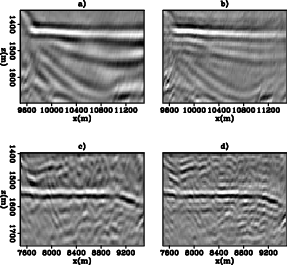
We apply LSRTM in two cases: (1) using the mirror-imaging operator (LSRTM-M) and (2) using the higher-order mirror-imaging operator (LSRTM-HM). The results after 10 iterations are shown in Figure 6 (c) and (d) respectively. Overall, the inversion images have higher resolution and fewer artifacts than the RTM image. However, there is not much difference between the two inversion results. One reason is that this dataset records only a small portion of the double-mirror signal. We expect the LSRTM-HM to provide substantial improvement in the case of a shallow-water dataset in which higher-order multiples overlap with lower order multiples. Comparing between RTM and LSRTM, we have identified two areas of improvement with some close-up sections in Figure 7:
|
|---|
|
Zoom
Figure 7. A section of the image cut from x=9400-11600 m and z=1350-1700 m after applying (a) RTM and (b) LSRTM-M. Another section of the image cut from x=7500-9500 m and z=1400-1750 m after applying (c) RTM and (d) LSRTM-M. |
|
|
|
|
|
|
Least-squares reverse time migration for the Cascadia ocean-bottom dataset |