next up previous [pdf]

Next: Discussion Up: Example Previous: Example 1: Complete baseline

Example 2: Complete baseline and Incomplete monitor data

Figure 9 shows that gapped monitor data. Here, we simulate an obstruction in the geometry such that neither sources nor receivers are present between $ 2500$ and $ 2900$ m. This gap in the the data coincides with the reservoir location. We image gapped monitor data using the same parameters and in the previous example. However, in order to warp this incomplete monitor to the complete baseline, we first perform Radon interpolation to fill in the monitor gap. The interpolated monitor data are then imaged and processed using the same parameters as in the complete monitor case. The resulting pre-stack image is then used to estimate the apparent displacement vectors (Figure 10) used to warp the incomplete monitor image to the baseline. The ratio of the Hessian diagonal (illumination ratio) between the baseline and monitor is shown Figure 11. Note that the region with low illumination ratios correspond to the location of the simulated obstruction. Figures 12 and 13 show the spatial and wavenumber domain point-spread-functions (PSFs) at point $ x=2600$ m and $ z=2600$ m, respectively. Note that there is significant differences in the PSFs away from the diagonal (center of the spatial PSF) and at various wavenumbers. Figure 14 shows the time-lapse images after different processing steps. Note the incremental improvements in the time-lapse image quality after processing and after inversion. Furthermore, note that compared to the complete data example (Figure 8(b)), the time-lapse image from conventional processing (Figure 14(b)) is of poorer quality.

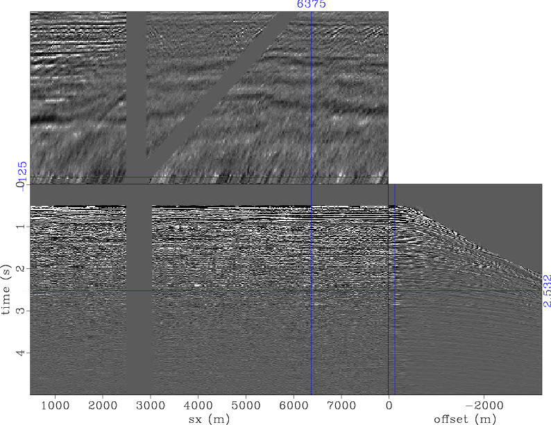
dmhl-dat-2759-b4-hole
Figure 9.
Gapped monitor data. Note that we have sources and receivers are missing around within the simulated obstruction.
[pdf] [png]

dmhl-warp-2759-08-rflat-ts
Figure 10.
Apparent vertical displacements between images from the baseline and interpolated monitor data sets. Comparing this to Figure 5, note that estimates of the apparent displacements are similar to those from the complete data case.
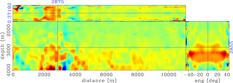
[pdf] [png]

hs-2759-rat
hs-2759-rat
Figure 11.
Illumination ratio between the baseline and monitor. Red indicates regions with equal illumination (i.e., ratio equals unity) whereas blue indicates unequal illumination (i.e., ratio less than unity).
[pdf] [png]

hs-2759-offd-06 hs-2759-offd-08 hs-2759-offd-diff
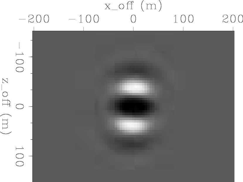
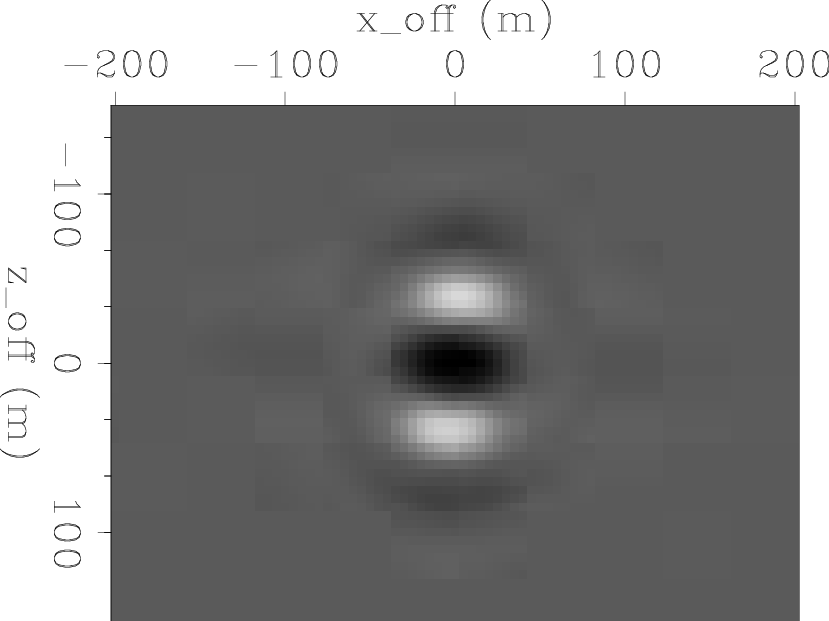
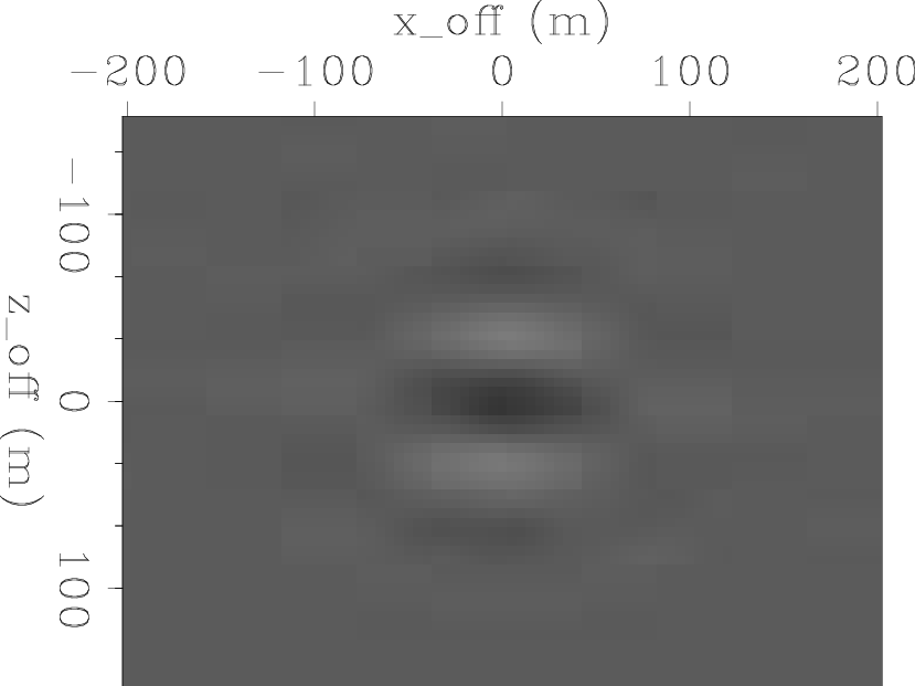
hs-2759-offd-06,hs-2759-offd-08,hs-2759-offd-diff
Figure 12.
Point-spread-functions at point $ x=2600$ m and $ z=2600$ m for the (a) baseline and (b) monitor. Note in the difference PSF (c), that there is significant energy away from the center of the PSF (i.e. in the off-diagonal parts of the Hessian).
[pdf] [pdf] [pdf] [png] [png] [png]

hs-2759-fft-06 hs-2759-fft-08 hs-2759-fft-diff
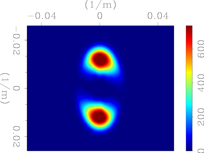
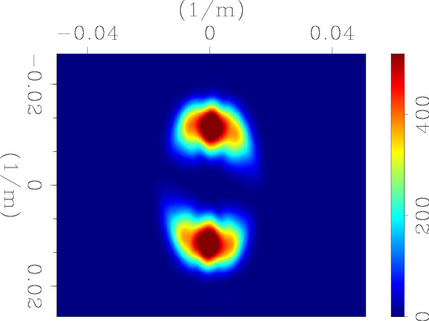
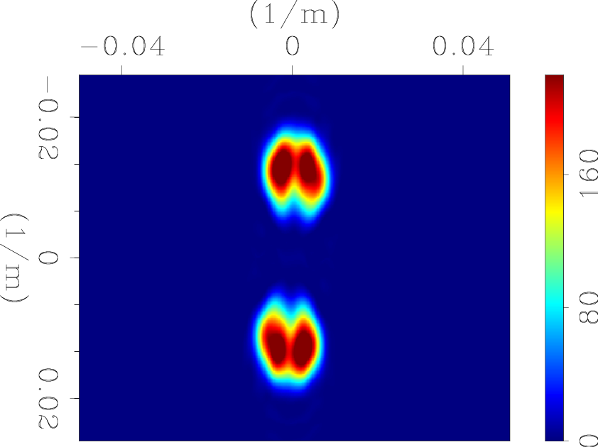
hs-2759-fft-06,hs-2759-fft-08,hs-2759-fft-diff
Figure 13.
Wavenumber domain point-spread-functions at point $ x=2600$ m and $ z=2600$ m for the (a) baseline and (b) monitor. Note in the difference PSF (c), that there is significant illumination differences at various wavenumbers.
[pdf] [pdf] [pdf] [png] [png] [png]

dmhl-raw-2759-4d dmhl-rwarp-2759-4d dmhl-inv-2759-4d
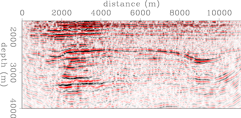
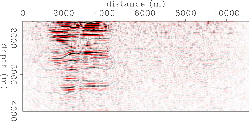
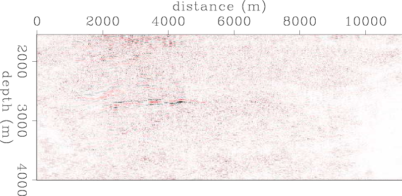
dmhl-raw-2759-4d,dmhl-rwarp-2759-4d,dmhl-inv-2759-4d
Figure 14.
Time-lapse images (a) from the raw data, (b) after time-lapse processing and (c) after wave-equation inversion. Also, because of artifacts introduced by the incomplete monitor data, conventional methods fail to provide results of comparable quality to the complete data example (Figure 8(b)). Note that inversion provides satisfactory results.
[pdf] [pdf] [pdf] [png] [png] [png]


next up previous [pdf]

Next: Discussion Up: Example Previous: Example 1: Complete baseline

2011-05-24