Wave-equation inversion of time-lapse seismic data sets

Example 1: Complete baseline and monitor data

Figure 2 shows the migrated pre-stack image obtained from the raw baseline data set. Note in Figure 2 that multiples show significant curvature relative to the correctly-migrated flat primaries. The same image after multiple attenuation is shown in Figure 3. In order to remove small velocities errors, we applied a residual moveout correction to the image gathers. The pre-processed pre-stack monitor image is shown in Figure 4. To obtain this image, in addition to the pre-processing applied to the baseline, we also applied a bulk amplitude correction to the monitor data. We estimate the amplitude correction as the ratio between the root-mean-square energy in the baseline versus the monitor. In addition, we perform pre-stack warping of the monitor to the baseline image. Apparent vertical displacements between the baseline and monitor are shown in Figure 5. Figure 6 shows the Hessian diagonal for the target area. Local dip estimates obtained from the stacked baseline image (not shown) are shown in Figure 7. Figure 8 shows the time-lapse images after different processing steps. Note the incremental improvements in the time-lapse image quality after processing and after inversion.

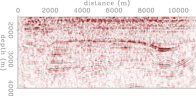
raw-2759-06
Figure 2. Raw pre-stack baseline image for the target area. Note the presence of several multiples and other undesired artifacts.

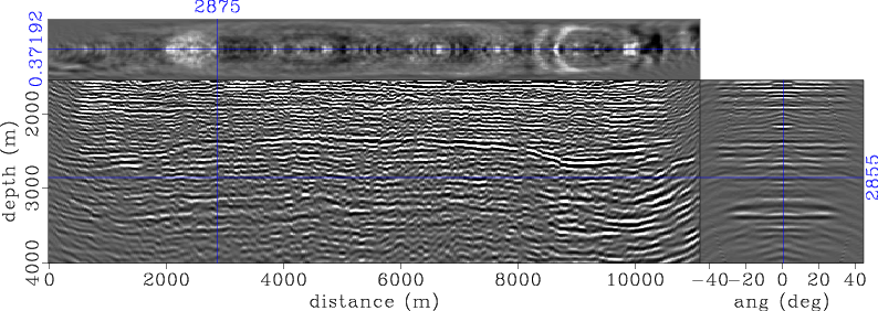
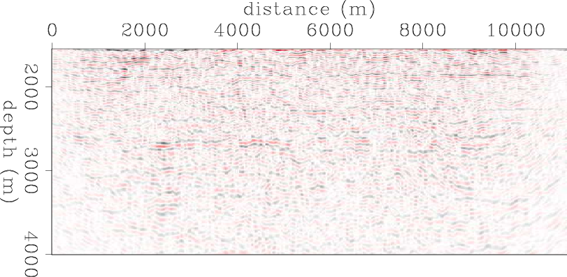
flat-2759-06-s
Figure 3. Preprocessed pre-stack baseline image of the target area. Note that the artifacts in the raw image (Figure 2) have been attenuated.

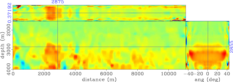
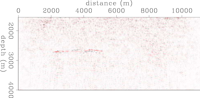
warp-2759-08
Figure 4. Preprocessed pre-stack monitor image of the target area obtained using the same parameters as in the baseline (Figure 3). Note that this image has been warped (using apparent displacements in Figures 5) to the baseline image.

warp-2759-08-rflat-ts
Figure 5. Apparent vertical displacements between the baseline and monitor images (Figures 3 and 4). Red, blue and green denote positive, negative and zero displacements respectively. Note that the maximum apparent displacements correspond to the reservoir location between position $2000$ m to $3000$ m. Also, note that the apparent displacement varies with opening angle.

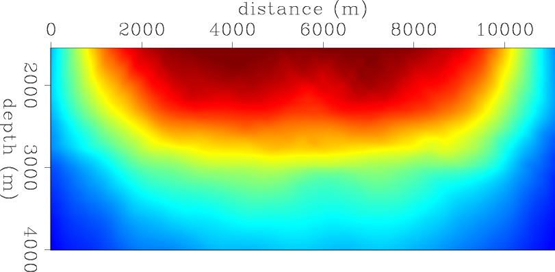
hs-2759-06
Figure 6. Illumination (Hessian diagonal) for the target area. Red indicates high illumination whereas blue indicates low illumination.

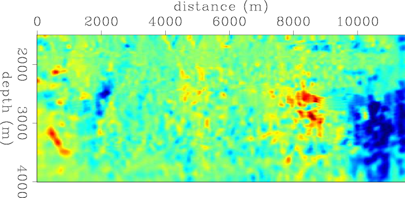
dm-dip-2759
Figure 7. Dip estimates obtained from the stacked baseline image. Red indicates positive dips whereas blue indicates negative dips. These dip estimates are used to construct the spatial regularization operator.

raw-2759-4d,rwarp-2759-4d,inv-2759-4d
Figure 8. Time-lapse images (a) from the raw data, (b) after time-lapse processing and (c) after wave-equation inversion. Note the incremental improvements in the time-lapse image from (a) to (c).

Wave-equation inversion of time-lapse seismic data sets