A new bidirectional deconvolution method that overcomes the minimum phase assumption

Inverting a 2D field section

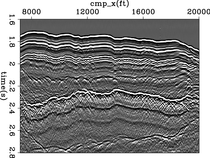
data-COF
Figure 7. Input Common Offset data.

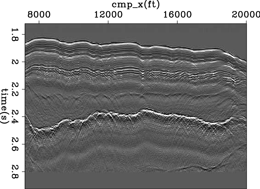
mod-COF-decon-old,mod-COF-decon
Figure 8. Given the common offset data in Figure 7, (a): reflectivity model retrieved from the original method; (b): reflectivity model retrieved from the bidirectional deconvolution method.

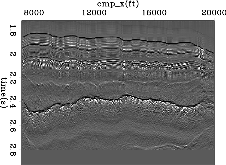
sm-integ-mod-COF-decon
Figure 9. Causal time integration of the reflectivity in figure 8(b). This should be the impedence.

The second example is a common-offset section of marine field data. Figure 7 shows the input data. Figure 8(a) shows the result using the old method. Figure 8(b) shows the result using the bidirectional deconvolution method.

The raw data in Figure 7 shows strong events like a double ghost (black, white, black). The traditional PEF result in Figure 8(a) shows strong events like doublets (black, white). The bidirectional deconvolution result in Figure 8(b) shows strong events like singlets (white). Examining Figure 8(b) we notice events at about 1.85s (black), 1.95s (black), 2.3s (white), 2.4s(black), 2.5s (mixed), and 2.8s (white). The unipolarity of individual suggests that a causal integration would produce the step functions we associate with impedence in a blocky model. Figure 9 is a first attempt to compute the impedence from the reflectivity in Figure 8(b). This was done by causal integration and some horizontal smoothing. Ideally, Figure 8(b) has only isolated white events and black events defining geologic boundaries. Time integrating these impulsive events should yield positive rectangle functions. Actually, the result we see in Figure 9 looks more like leaky integration of Figure 8(b). The small events present in Figure 8(b) apparently contains low frequency energy at the opposite polarity of that of the isolated impulses. We could thus regard Figure 9 as a failure. Instead we regard it as an inverse problem that we have not yet correctly posed. The failure arises because the raw data fails to contain the required low frequencies. Were we to replace small values in Figure 8(b) by zeros, we might have obtained a result more to our liking. We need to formalize the inverse problem and reduce it to the usual situation which is how much to regard the data as perfect, and how to allow imperfection to be overcome by methodology that tends us to blocky models.

A new bidirectional deconvolution method that overcomes the minimum phase assumption