|
|
|
|
Implementing implicit finite-difference in the time-space domain using spectral factorization and helical deconvolution |
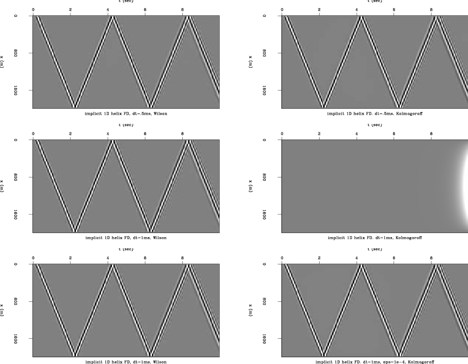
This result indicates that the Kolmogoroff factorization method is even less suitable than the Wilson method for this finite-difference scheme, since the addition of a small value to the central FD coefficient when using Wilson is necessary only at greater time step sizes.
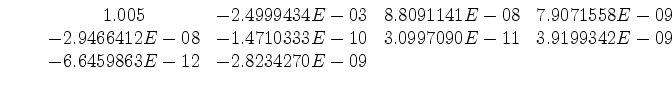
The ten Wilson filter coefficients used to create the center panels in Figure 10 were:
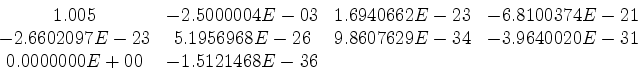
The Kolmogoroff coefficients were:
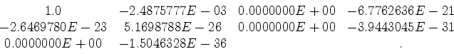 |
Other than the zero-lag coefficient not being equal to 1, a striking difference is that the Kolmogoroff coefficients do not drop off quickly as do the Wilson coefficients. This has a degrading effect on the filter correlation. The Wilson filter's correlation is:
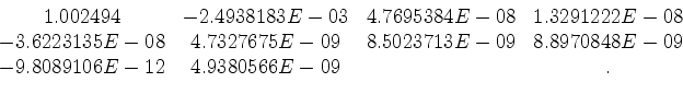 |
The Kolmogoroff's filter correlation is:
 |
The finite-difference coefficients for the parameter set of the wavefields in Figure 10 are
 . The Wilson filter's correlation recreates these weights precisely, while the Kolmogoroff filter's correlation does not. Also, the drop-off in the magnitude of the filter correlation at lags which do not represent finite-difference weights (i.e. not lag 0 or lag 1) is much better for the Wilson filter.
|
|---|
|
wil-vs-kol
Figure 10. 1D helical implicit finite-difference with Wilson-Burg spectral factorization (left), and Kolmogoroff spectral factorization (right). |
|
|
|
|
|
|
Implementing implicit finite-difference in the time-space domain using spectral factorization and helical deconvolution |