Seismic reservoir monitoring with encoded permanent seismic arrays

Conclusions

A method for reservoir monitoring with encoded data from permanent seismic arrays has been proposed. Encoding randomly delayed intermittent sweeps from low-energy sources reduces the total recording time for each seismic experiment. Direct imaging of such data give good-quality images that can be used for near-continuous reservoir monitoring. The numerical experiment shows that seismic amplitude and geomechanical changes from the proposed method are similar to those from conventional seismic data.

pmigN1,pmigN2,pmigN3,pmigN4,pmigN5
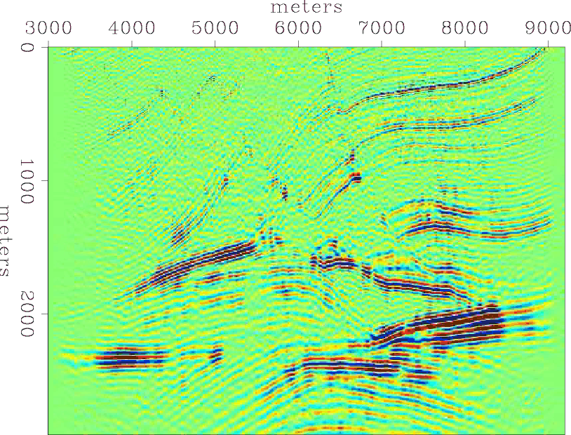
Figure 5. Images from shot-profile imaging of noise-free conventional data over five models modified from Figure 3.

pmig0n-6-1,pmig2n-6-2,pmig2n-6-3,pmig2n-6-4,pmig2n-6-5
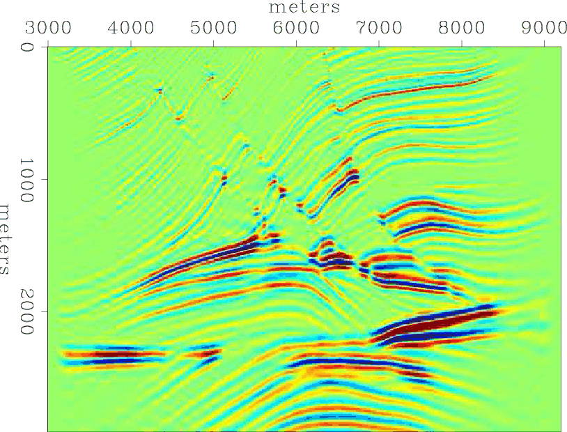
Figure 6. Images from direct imaging of $6$ seconds encoded intermittent source data (Figure 4). Note the presence of numerous crosstalk and ambient noise artifacts.

pmig0n-288-1,pmig2n-288-2,pmig2n-288-3,pmig2n-288-4,pmig2n-288-5
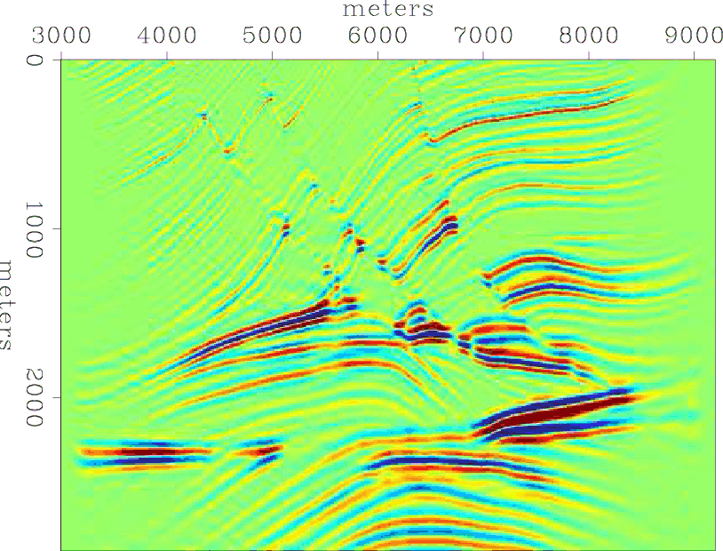
Figure 7. Images from direct imaging of $320$ seconds of encoded intermittent sweep data (Figure 4). Note that the crosstalk and ambient noise artifacts in Figure 6 have been attenuated. Note that these images are comparable to those in Figure 5.

pmig0n-288-4d-2,pmig0n-288-4d-3,pmig0n-288-4d-4,pmig0n-288-4d-5
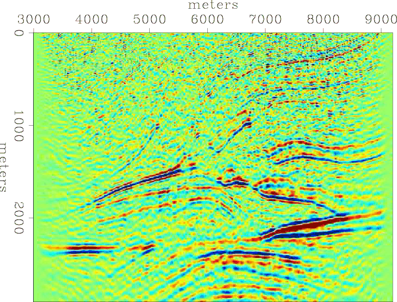
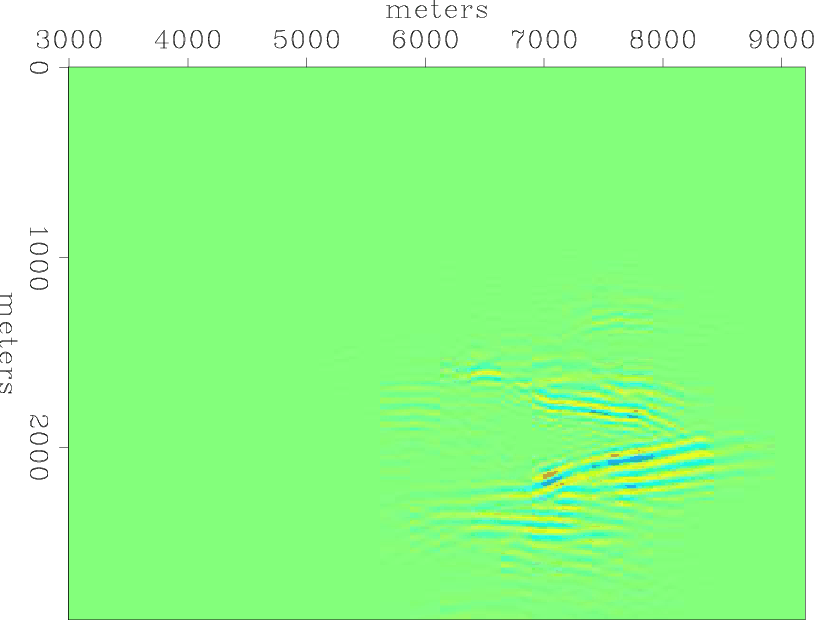
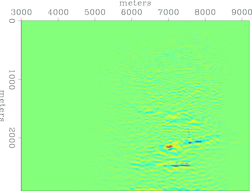
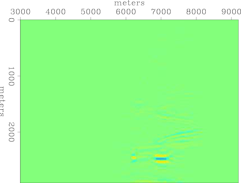
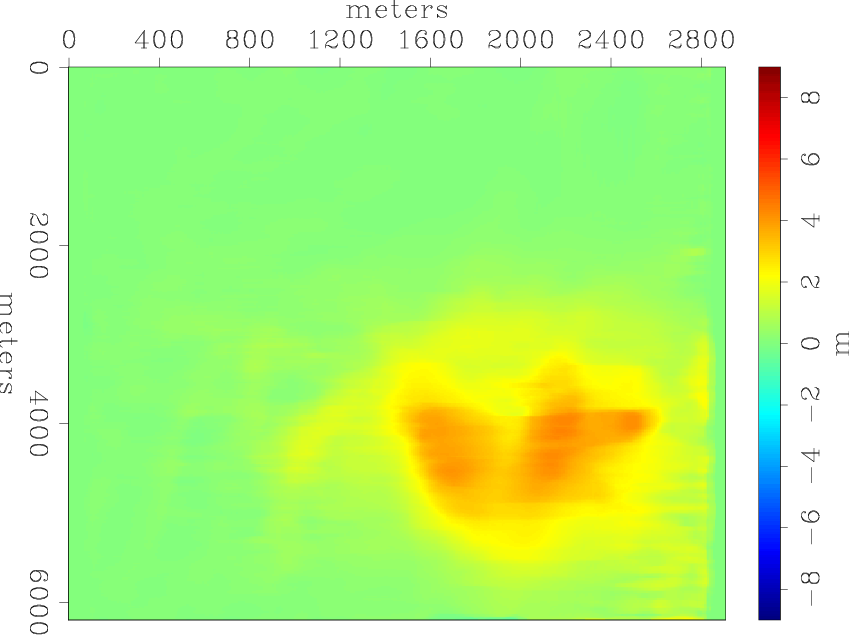
Figure 8. Time-lapse images from direct imaging of encoded intermittent source data (Figure 4). Note that the seismic amplitude changes at the reservoir are masked by the strong misalignment of the images which result from migration with a wrong baseline velocity. Reservoir change increases non-linearly from top to bottom.

pmig1n-288-4d-2,pmig1n-288-4d-3,pmig1n-288-4d-4,pmig1n-288-4d-5
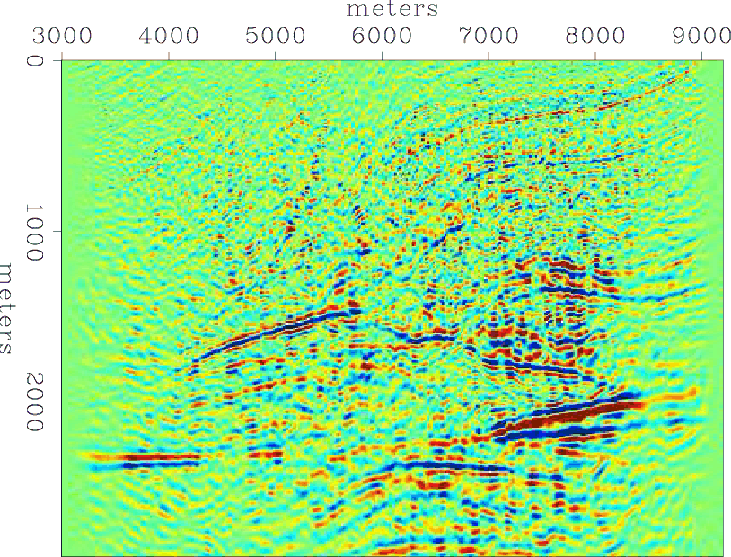
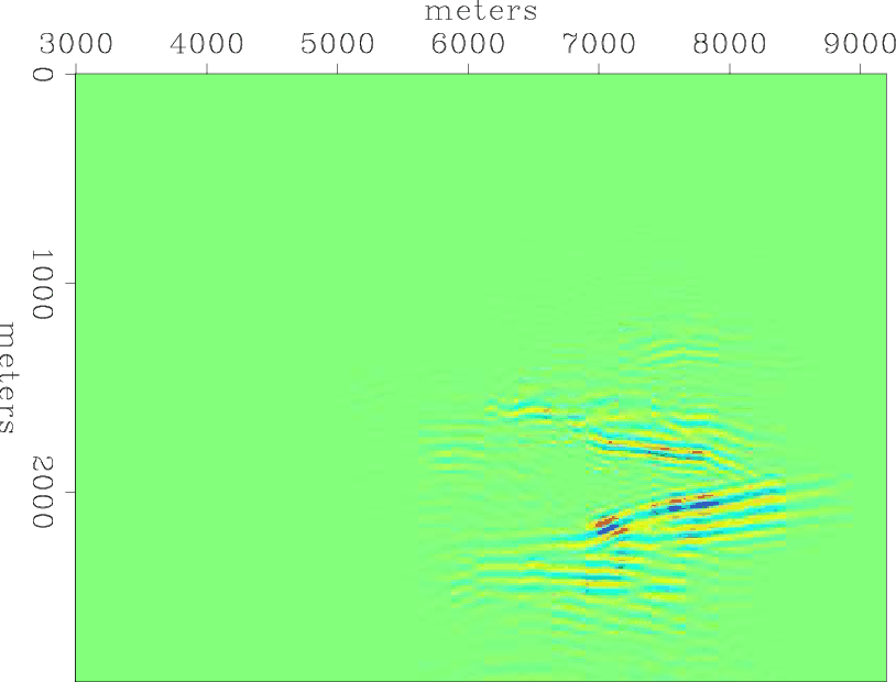
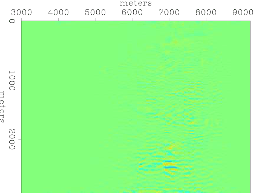
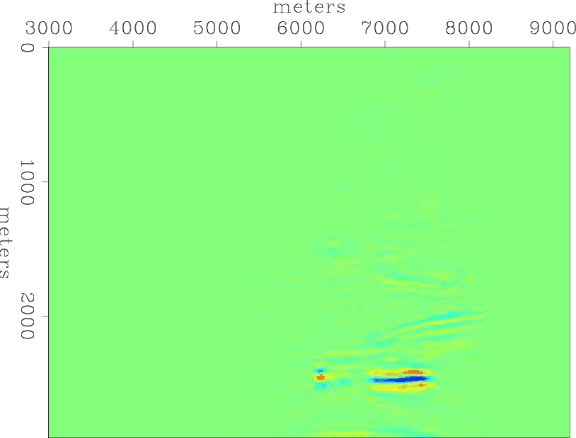
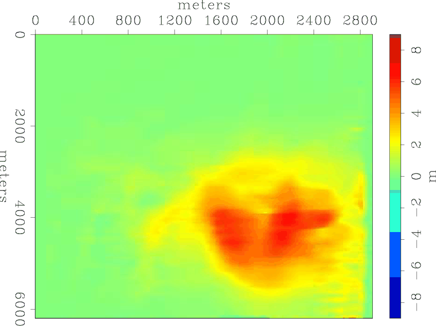
Figure 9. Time-lapse images from direct imaging of encoded intermittent source data (Figure 4) after cyclic 1D warping to remove image misalignments. Note that the seismic amplitude changes at the reservoir are better clearly defined than in Figure 8. However some artifacts (e.g. from the over-hanging salt wedge) persist.

pmig2n-288-4d-2,pmig2n-288-4d-3,pmig2n-288-4d-4,pmig2n-288-4d-5
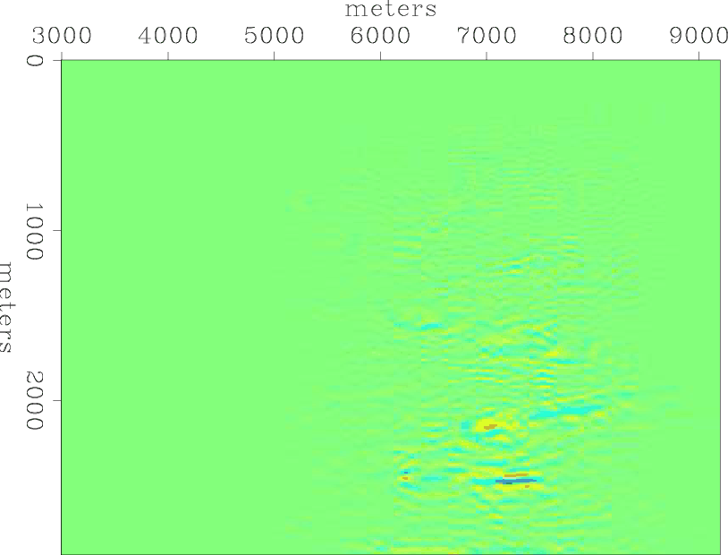
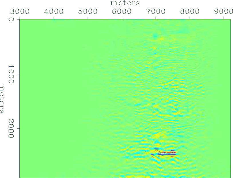
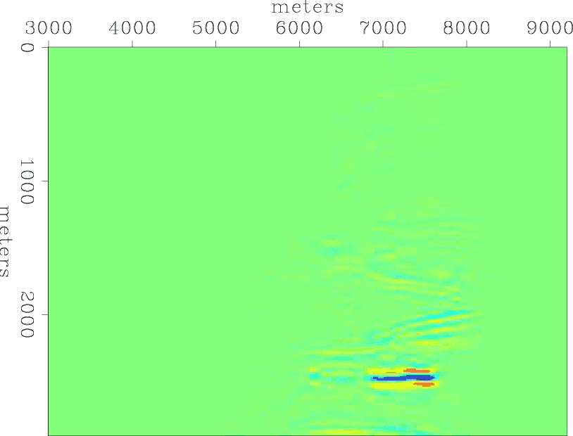
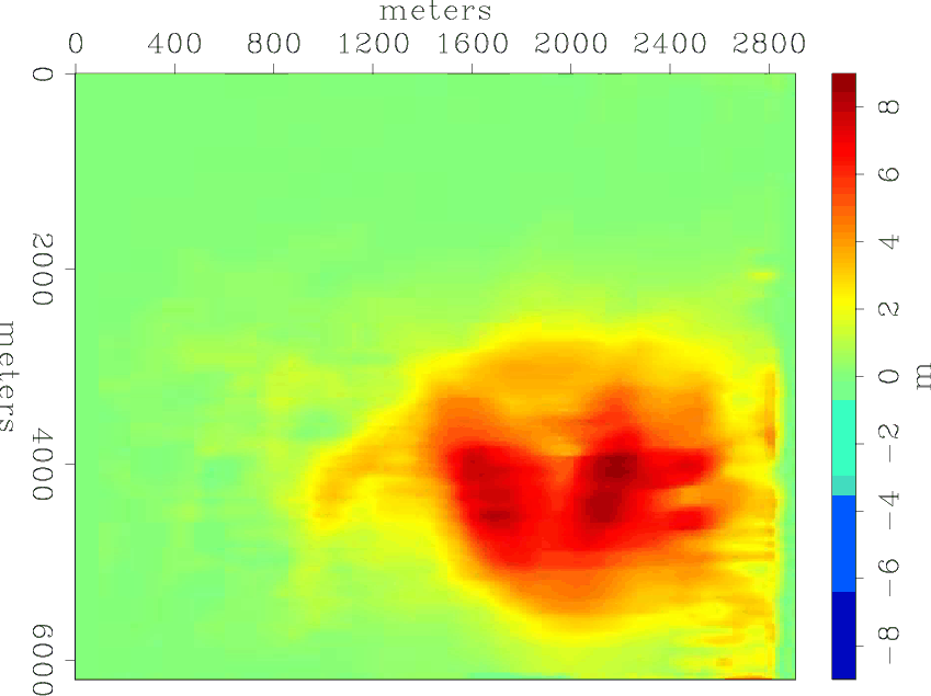
Figure 10. Time-lapse images from direct imaging of encoded intermittent source data (Figure 8) after match-filtering to remove residual artifacts. Compare this to Figures 8 and 9. Note that the seismic amplitude change (and discontinuities) are accurately imaged by the proposed method.

pmigN-4d-2,pmigN-4d-3,pmigN-4d-4,pmigN-4d-5
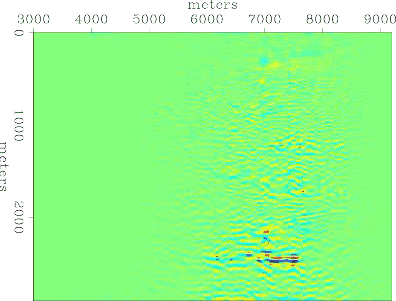
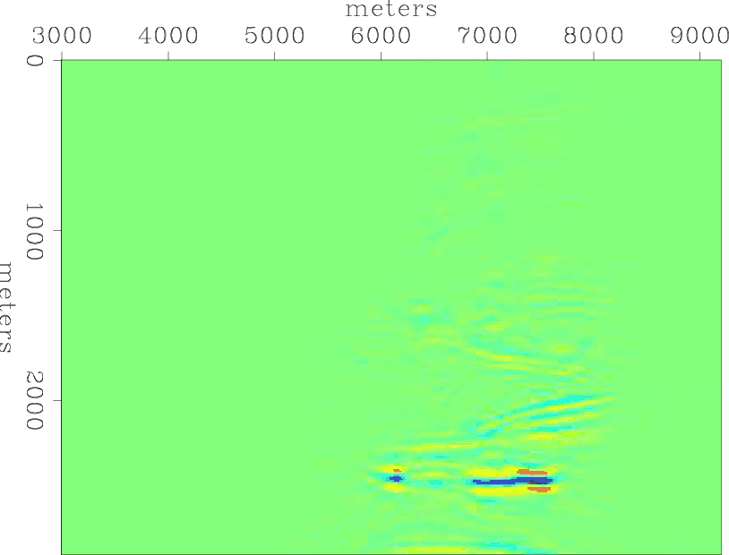
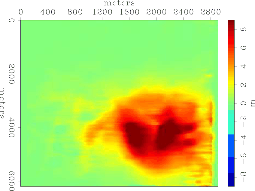
Figure 11. Time-lapse images from from conventional (single-source, high-energy, shot-period) seismic data after warping and match-filtering. These results were obtained using the same models as in the intermittent-source case. Note that these results are similar to those from the proposed method (Figure 10).

ptsn-288-2,ptsn-288-3,ptsn-288-4,ptsn-288-5
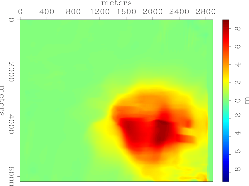
Figure 12. Vertical components of the apparent displacement vectors computed by warping the monitor images in Figure 7 to the Baseline (Figure 7(a)). Note that these are similar to those from conventional data recording/processing (Figure 13).

ptsn2,ptsn3,ptsn4,ptsn5
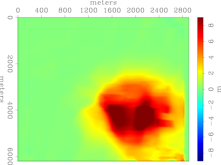
Figure 13. Vertical components of the apparent displacement vectors computed by warping the monitor images in Figure 5 to the Baseline (Figure 5(a)). Note that, in general, these are similar to those from the proposed method (Figure 12).

Seismic reservoir monitoring with encoded permanent seismic arrays