Seismic reservoir monitoring with encoded permanent seismic arrays

Numerical example

Five data sets were modeled over a modified section of the 2D Marmousi model (Figure 3). The objective is to image seismic amplitude and geomechanical changes around the reservoir using encoded data sets from permanent arrays. Non-linear, discontinuous changes in the reservoir were modeled by velocity changes within the reservoir. Geomechanical changes due to reservoir compaction were modeled by a morphed expanding gaussian anomaly above the reservoir.

vel-1
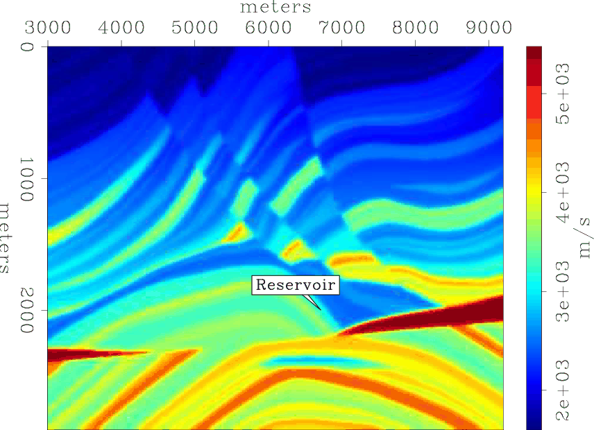
Figure 3. 2D Marmousi velocity model.

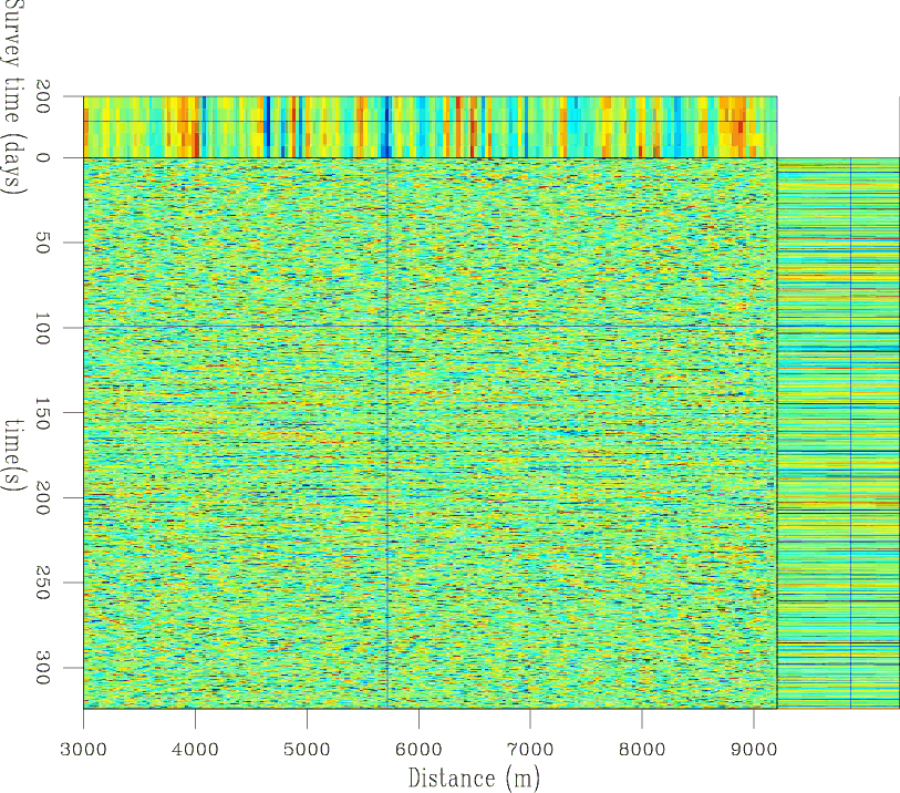
Each surface seismic source generates an intermittent sweep within a six-second window with unique random zero- to three-second delays between sources. $320$ seconds of data from ${388}$ seismic sources were recorded by surface receivers (Figure 4). Although it was not essential, because this method allows for perfect repeatability, the same encoding function was used for all surveys. However, different amounts of ambient noise (coherent plane-wave and uniform-distribution random noise) were introduced for each survey to produce data at S/N of 4:1. For each survey, using a strongly smoothed version of the baseline modeling velocity, all data were imaged directly with a phase-encoding one-way wave equation algorithm. For comparison, images from noise-free conventional data and processing are shown in Figure 5, those from only $6$ seconds of data are shown in Figure 6, and those from the full $320$ seconds of data are shown in Figure 7. Note that the longer data records (Figure 7) produce cleaner images than the shorter data records (Figure 6). Note that in the encoded data examples, only a single phase encoded shot-profile migration was required for each survey.

Time-lapse images computed from the migrated images show significant misalignments (Figure 8). Results obtained after alignment and after match filtering are shown in Figures 9 and 10. Note that time-lapse images obtained after matching are comparable to those obtained from the conventional example (Figure 11). In addition, note that apparent displacements--which carry geomechanical information--estimated from the proposed method (Figure 12) and from conventional methods (Figure 13) are similar.

pdatn288
Figure 4. Five seismic data sets from intermittent seismic sweeps over the model in Figure 3. The intersecting lines indicate positions of the three panels within the data volume.

Seismic reservoir monitoring with encoded permanent seismic arrays