 |
 |
 |
 | A preconditioning scheme for full waveform inversion |  |
![[pdf]](icons/pdf.png) |
Next: Preconditioning
Up: Guitton and Ayeni: Preconditioned
Previous: Introduction
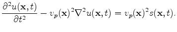
In this paper, we use a time domain approach for solving the scalar acoustic wave equation (parametrized in terms of P-wave velocity  ):
):
 |
(3) |
with the source term
 where
where 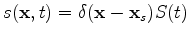 is the source function at
 and
and
 the pressure field.
Tarantola (1984) derives the expression of the gradient for the acoustic equation (3) for each component of
the pressure field.
Tarantola (1984) derives the expression of the gradient for the acoustic equation (3) for each component of
 (equal to
only in this case).
(equal to
only in this case).
 |
(4) |
where
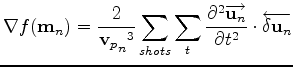 is the backward propagated residual at iteration
  such that
 and
and
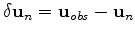 is the forward propagated synthetic source.
For our iterative method, we opted for the L-BFGS approach of Nocedal (1980).
This quasi-Newton approach computes an estimate of the inverse Hessian iteratively by using a user-defined number of solution and gradient vectors.
One of the main benefits of this technique is that because the Hessian is never explicitely formed, there is significant computational and memory savings. W
ith the L-BFGS solver, the model is updated as follows:
is the forward propagated synthetic source.
For our iterative method, we opted for the L-BFGS approach of Nocedal (1980).
This quasi-Newton approach computes an estimate of the inverse Hessian iteratively by using a user-defined number of solution and gradient vectors.
One of the main benefits of this technique is that because the Hessian is never explicitely formed, there is significant computational and memory savings. W
ith the L-BFGS solver, the model is updated as follows:
 |
(5) |
where
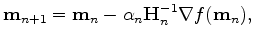 is the updated solution,
  the step length computed by a line search
that ensures a sufficient decrease of
the step length computed by a line search
that ensures a sufficient decrease of
 and
and
 the approximate Hessian. To improve chances of not falling into a local minimum, we
follow a multi-scale approach (Bunks et al., 1995) where the source and data are bandpassed prior to inversion. We introduce our preconditioning scheme
in the following section.
the approximate Hessian. To improve chances of not falling into a local minimum, we
follow a multi-scale approach (Bunks et al., 1995) where the source and data are bandpassed prior to inversion. We introduce our preconditioning scheme
in the following section.
|
|
|
|
| A preconditioning scheme for full waveform inversion | |
|
Next: Preconditioning
Up: Guitton and Ayeni: Preconditioned
Previous: Introduction
2010-11-26