A preconditioning scheme for full waveform inversion

Introduction

The goal of waveform inversion is to derive physical properties of the Earth, such as P-wave velocity, S-wave velocity, or density. These properties can be related to the presence of hydrocarbons in the subsurface and their estimation is one of the most important goal in seismic processing. In practice, we try to minimize the function

$$f(\textbf{m})= \Vert \textbf{u}_{obs} - \textbf{u}_{mod} \Vert ^ {norm}$$ (1)

where $\textbf{m}$ is a vector of physical properties (what we are looking for), $\textbf{u}_{obs}$ the observed and $\textbf{u}_{mod}$ the modeled data. Note that $f$ is a 1-D function defined by the choice of a norm. In practice, the $\ell^2$ norm is often chosen, but the $\ell^1$ norm seems to have more practical needs for its robustness to non-Gaussian noise present in the data (Crase et al., 1990). The minimization of $f(\textbf{m})$ can be achieved using iterative methods. Tarantola (1984) establishes that the model can be updated as follows:

$$\textbf{m}_{n+1} = \textbf{m}_{n}-\alpha_n.\nabla f(\textbf{m}_n)$$ (2)

where $\nabla f(\textbf{m})$ is the gradient of $f(\textbf m)$ and $\alpha_n$ a step-length that needs to be estimated. It turns out that the computation of the gradient is equivalent to a reverse-time migration (Lailly, 1984).

Unfortunately, although a promising approach, waveform inversion is hampered by many issues. The main one is the presence of local minima in $f$ . To circumvent this problem, the data can be inverted in a multi-scale fashion in the time (Bunks et al., 1995) or frequency domain (Sirgue and Pratt, 2004). Furthermore, time damping of the input data offers opportunities to focus the inversion on different parts of the data, thus reducing the effects of local minima (Brenders et al., 2009).

Traditionally, ill-posed problems can be solved by adding a regularization term to the objective function. Very often, a regularization term that can penalize differences between neighboring points is selected. However, whereas waveform inversion tends to add details to a velocity model, regularization tends to smooth them out, thus working against our primary goal: fitting the data. One way to address these somewhat conflicting goals is to use preconditioning. Here, we show how we can geologically constrain the velocity model by using a non-stationary preconditioning approach. This method requires two ingredients: a dip estimation method and a local dip filtering technique. We use the method of Fomel (2002) for the former and of Hale (2007) for the later.

In this paper we first introduce the waveform inversion approach, with and without preconditioning. We show that preconditioning amounts to a simple change of variable which, in effect, changes the gradient direction. Then, we present our method of local dip filtering, which follows Hale's. Finally, we present synthetic results on a modified version of the Marmousi model. These results demonstrate that non-stationary, preconditioned inversion yields geologically plausible models.

MarmLapSEG
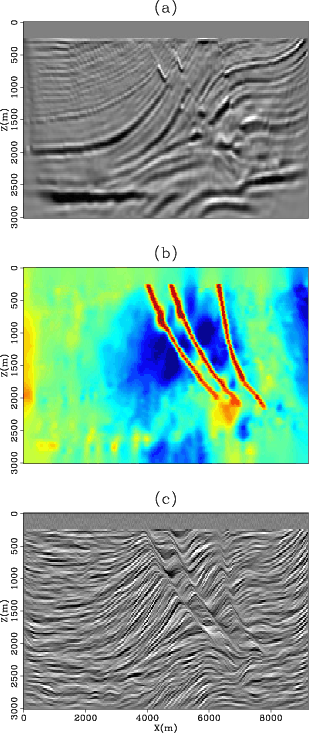
Figure 1. Illustration of the preconditioning operator $\mathbf{S}$ . We first migrate the synthetic Marmousi dataset to obtain (a). Then, suing the migrated image, we compute the dip field (b). In this example, faults are picked by hand and smoothed horizontally to preserve discontinuities in the velocity model. Applying $\mathbf{S}$ built from (b) to a random field shows in (c) the texture of the migrated section in (a). Note how the water-column is not smoothed and how the fault locations are clearly visible.

MarmWVISEG
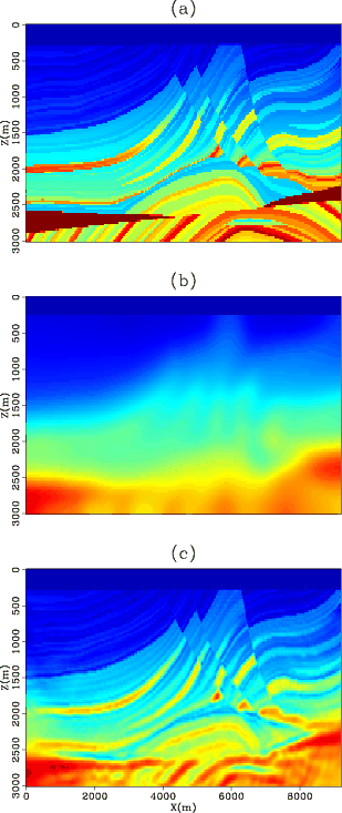
Figure 2. (a) True velocity model used to generate the synthetic dataset. (b) Initial guess obtained by smoothing the true model in (a). (c) Estimated model after waveform inversion. No preconditioning is applied in this case. Four frequency bands were used to bandpass both the source and the data prior to inversion (0-4Hz, 0-8Hz, 0-12Hz, 0-16Hz). The velocity model is recovered very well.

A preconditioning scheme for full waveform inversion