next up previous [pdf]

Next: Conclusions Up: Almomin and Tang: WEMVA Previous: Interpretation

Synthetic Examples

Although the derivation was performed in the frequency-domain, we will apply the tomographic operator in the time-domain. First, we will start with a simple example with a constant background velocity of 2500 m/s. The spatial sampling is 10 m and the temporal sampling is 2 ms. A Ricker wavelet with a fundamental frequency of 20 Hz is used to model the data. There is one reflector at the bottom of the model at a depth of 900 m. Now, we will input a slowness perturbation to the forward operator to generate a corresponding image perturbation. Three slowness perturbations are supplied. First, a spike located at a depth of 400 m. Second, a vertical line extending from a depth of 300 m to 500 m. Third, a horizonal line at a depth of 400 m. The three slowness perturbations are shown in Figure 1.

deltaS
deltaS
Figure 1.
Three slowness perturbations that will be used in the forward operator.
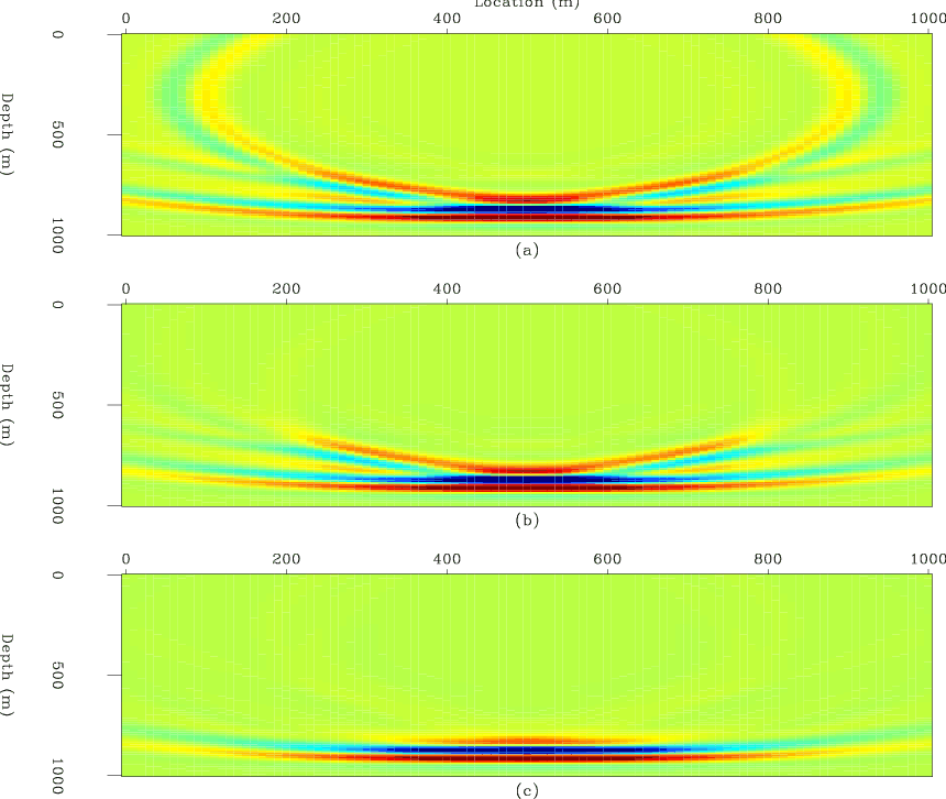
[pdf] [png]

We apply the forward tomographic operator on these slowness perturbations to get the corresponding image perturbations. Figure 2 shows the image perturbation (at zero subsurface offset only).

deltaI
deltaI
Figure 2.
The three image perturbations corresponding to slowness perturbations in Figure 1, produced by the forward scattering operator.
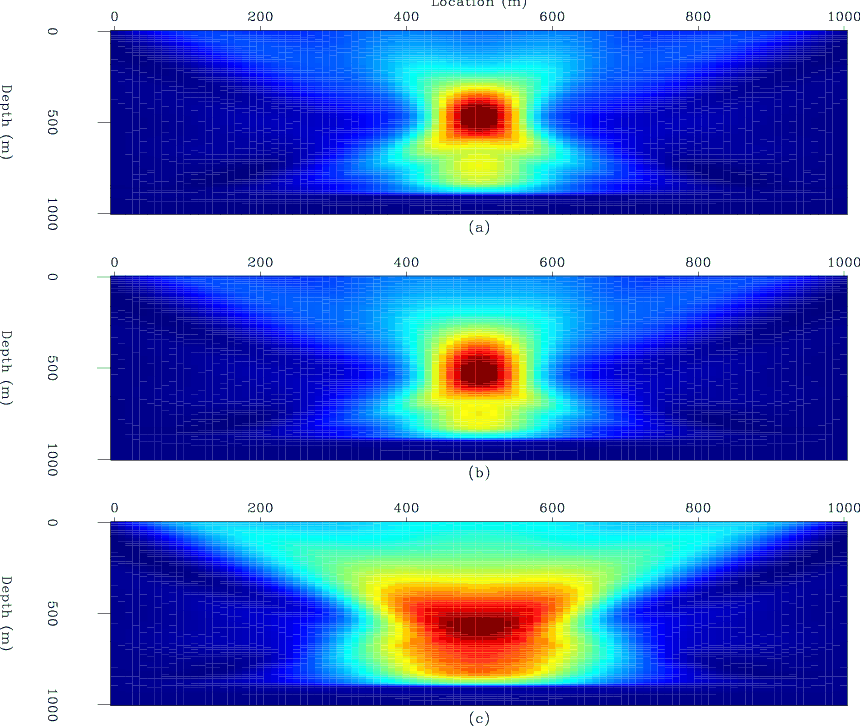
[pdf] [png]

Then, we apply the adjoint tomographic operator to these image perturbations to recreate the slowness perturbations. The results of applying the adjoint scattering operator are shown in Figure 3. As expected, the reconstructed slowness perturbations have higher horizontal resolution than vertical resolution.

deltaS2
deltaS2
Figure 3.
The reconstructed slowness perturbations by the adjoint scattering operator.
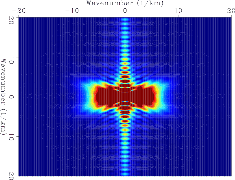
[pdf] [png]

Figure 4 shows the amplitude spectrum of the recreated slowness perturbation in Figure 3(a).

spect
spect
Figure 4.
The Fourier transform of spike response in Figure 3(a).
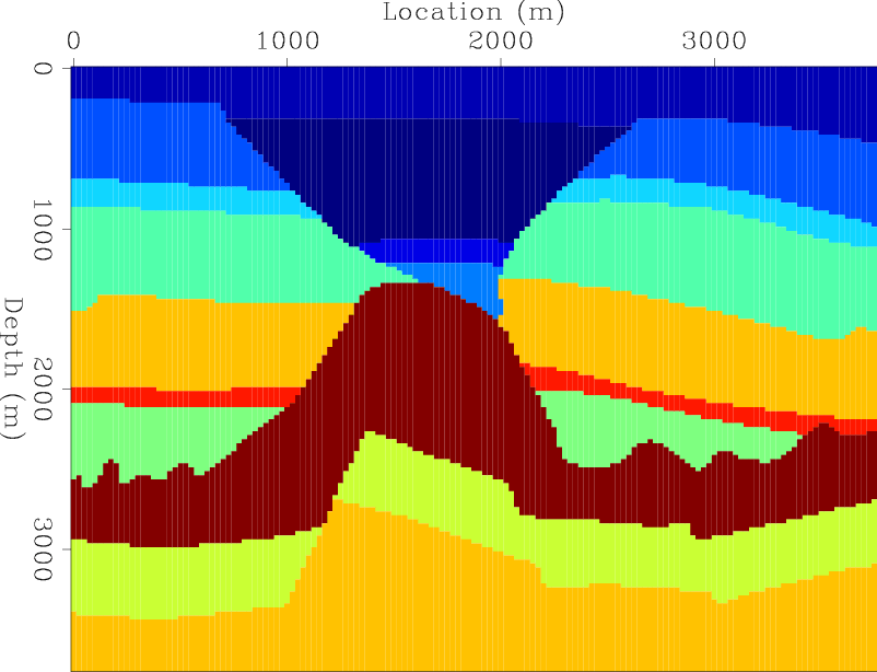
[pdf] [png]

For a second test, we will repeat a similar experiment but with a different background velocity model. As shown in Figure 5, the velocity model includes areas of low velocity to the top, and areas of high velocity in the middle, representing a salt body. There is one reflector at the bottom of the model at a depth of 3500 m.

velbg3
velbg3
Figure 5.
The background velocity model for the second test.
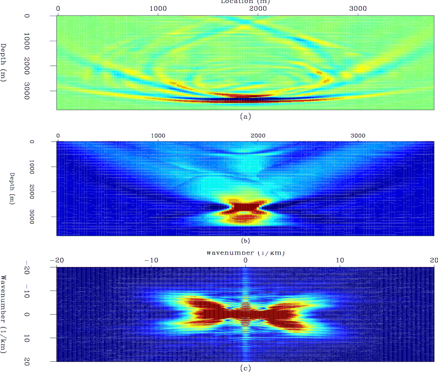
[pdf] [png]

The spatial sampling is 25 m and the temporal sampling is 4 ms. A Ricker wavelet with a fundamental frequency of 10 Hz is used to model the data. The slowness perturbation is a spike located at a depth of 2600 m, which is located in between the reflector and the salt body. The corresponding image perturbation resulted from applying the forward tomographic operator is shown in Figure 6(a) and the reconstructed slowness perturbation is shown in Figure 6(b). Figure 6(c) shows the amplitude spectrum of the reconstructed slowness perturbation. The change in the background velocity affected the reconstructed slowness perturbation, both in physical space and in Fourier space.

results3
results3
Figure 6.
Using the background velocity in Figure 5, (a) the image perturbation, (b) reconstructed slowness perturbation, and (c) the Fourier transform for the reconstructed slowness perturbation.
[pdf] [png]


next up previous [pdf]

Next: Conclusions Up: Almomin and Tang: WEMVA Previous: Interpretation

2010-11-26