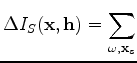
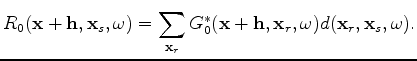
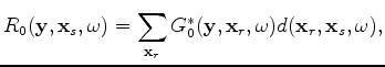
There are several ways to interpret equations (14) and (15). For simplicity, let us first break each perturbation into two components, one from the source side and one from the receiver side. So, for equation (14), the first component will be as following:
(16)
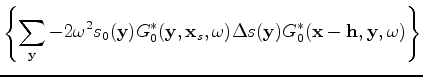
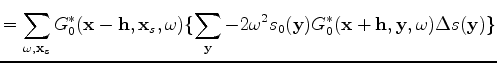
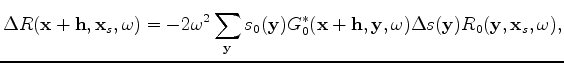
Now, we can further break equation (16) into two components that we define as follows:
(17)
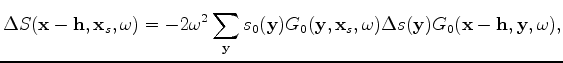
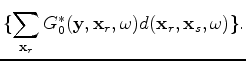
and
(18)
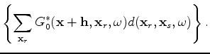
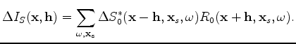
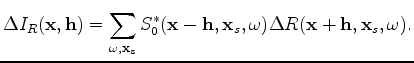
We can see that equation (17) represents the Born-modeled-wavefield due to the slowness perturbation and equation (18) represents the background receiver wavefield. So, we can now present the source side of the image perturbation as the following:
(19)
Now, we can perform a similar analysis on the other component of equation (14), which is:
(20)
Again, let us define a perturbed receiver wavefield and a background source wavefield as the following:
(21)
(22)
(23)
This enables us to represent the receiver side of the image perturbation as the following:
(24)
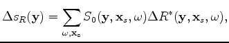
As for equation (15), we do the same analysis to arrive at the following gradient formulae:
(25)
(26)
where the residual wavefields are defined as the following:
(27)
(28)
In summary, the tomographic operator computes the image perturbation or slowness perturbation by correlating background and residual wavefields of both source and receiver sides.
Migration velocity analysis based on linearization of the two-way wave equation