|
|
|
|
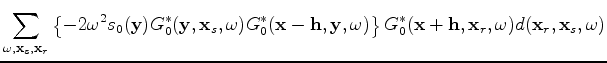
Migration velocity analysis based on linearization of the two-way wave equation |
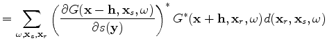
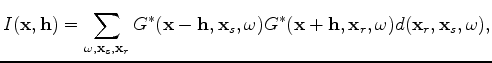 is the image,
with respect to the slowness as follows;
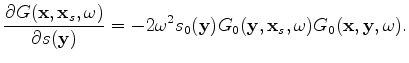
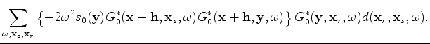
is the image,
with respect to the slowness as follows;
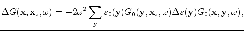
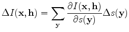
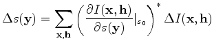
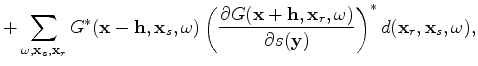 is the slowness coordinate. Now, we can perturb the slowness:
|
|
|
|
Migration velocity analysis based on linearization of the two-way wave equation |