|
 |
 |
 | Seismic reservoir monitoring with simultaneous sources |  |
![[pdf]](icons/pdf.png) |
Next: Numerical Example
Up: Ayeni: 4D simultaneous sources
Previous: Linear phase-encoded modeling and
For an arbitrary survey  , we can simplify the modeling equation into the form
 |
(4) |
where
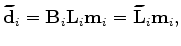 is the recorded data,
  is the encoding operator,
  is the modeling operator,
  is the earth reflectivity, and
 .
The migrated image, computed by applying the adjoint operator
.
The migrated image, computed by applying the adjoint operator
 to
, will contain cross-term artifacts generated by cross-correlation between incongruous source and receiver wavefields (Romero et al., 2000; Tang and Biondi, 2009).
In addition, because of the associated geometry and relative shot-time non-repeatability, different surveys have unique cross-term artifacts.
To attenuate these artifacts, for
to
, will contain cross-term artifacts generated by cross-correlation between incongruous source and receiver wavefields (Romero et al., 2000; Tang and Biondi, 2009).
In addition, because of the associated geometry and relative shot-time non-repeatability, different surveys have unique cross-term artifacts.
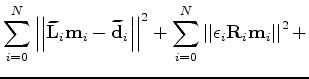
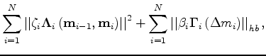
To attenuate these artifacts, for  surveys, we minimize a joint (global) cost function
  given by
where the parameters
 and
and  determine the strengths of the spatial and temporal regularization operators,
 and
and
 respectively.
Because only a small region in the model space contain desired in time-lapse signal, a sparseness requirement is desirable.
Parameter
respectively.
Because only a small region in the model space contain desired in time-lapse signal, a sparseness requirement is desirable.
Parameter  determines the strength of the sparseness operator
 .
Related formulations have been applied to other time-lapse imaging problems (Ajo-Franklin et al., 2005).
We compute the time-lapse image as the difference between the migrated or inverted image at time
.
Related formulations have been applied to other time-lapse imaging problems (Ajo-Franklin et al., 2005).
We compute the time-lapse image as the difference between the migrated or inverted image at time  and that at time 0
.
Because several shots are encoded and directly imaged, the computational cost of this approach is considerably reduced compared to non-encoded data sets.
and that at time 0
.
Because several shots are encoded and directly imaged, the computational cost of this approach is considerably reduced compared to non-encoded data sets.
In this paper, the spatial regularization operator is a system of non-stationary dip-filters, whereas the temporal regularization operator is a gradient between surveys.
We compute dips using the plane-wave destruction method (Fomel, 2002), and we compute dip-filters using factorized directional Laplacians (Hale, 2007).
To ensure stable transitions at sharp boundaries, the filter corresponding to any image point is scaled according to a dip-contrast-dependent variance.
We estimate the spatial and temporal regularization parameters by scaling the maximum amplitude in each data set.
Finally, we minimize the objective function using an iterative hybrid conjugate direction algorithm (Li et al., 2010) which enforces desired spareness on the time-lapse images.
|
|
|
|
| Seismic reservoir monitoring with simultaneous sources | |
|
Next: Numerical Example
Up: Ayeni: 4D simultaneous sources
Previous: Linear phase-encoded modeling and
2010-05-19