 |
 |
 |
 | Seismic reservoir monitoring with simultaneous sources |  |
![[pdf]](icons/pdf.png) |
Next: Regularized joint inversion
Up: Ayeni: 4D simultaneous sources
Previous: Introduction
From the linearized Born approximation of the acoustic wave equation, the seismic data  recorded by a receiver at
 due to a shot at
 is given by
 |
(1) |
where 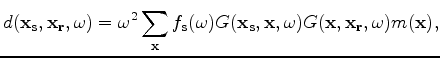 is frequency,
 is the reflectivity at image points
  ,
,
 is the source wavelet,
and
is the source wavelet,
and
 and
and
 are the GreenÕ's functions from
to
and from
to
, respectively.
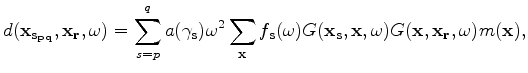
When there are multiple seismic sources, the recorded seismic data is due to a concatenation of phase-shifted sources.
For example, the recorded data due to shots starting from
are the GreenÕ's functions from
to
and from
to
, respectively.
When there are multiple seismic sources, the recorded seismic data is due to a concatenation of phase-shifted sources.
For example, the recorded data due to shots starting from  to
to  , is given by
 |
(2) |
where
 is given by
 |
(3) |
and
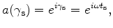 , the time-delay function, depends on the delay time
  at shot
  .
.
For acquisition efficiency, it is unnecessary to repeat either the acquisition geometry or the relative shot timings for different surveys.
By eliminating the cost associated with repeatability between surveys, we can significantly reduce the total acquisition cost.
Because acquisition cost is usually several times higher than the processing cost, a reduction in acquisition cost will significantly reduce the total seismic monitoring cost.
In addition, we achieve further cost reduction by imaging all the data sets directly.
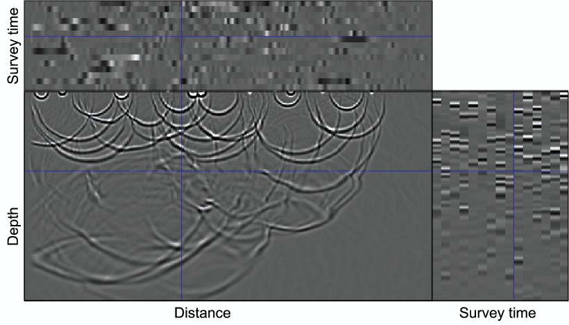
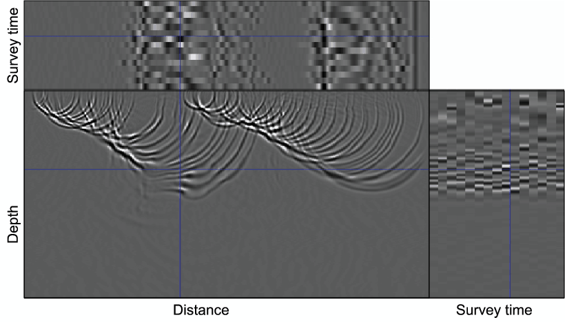
Figure 2 shows examples of wavefields from two configurations of simultaneous-shooting.
In both figures, the third dimension represents the survey time, while the orthogonal lines indicate positions of the displayed slices within the cube.
|
|---|
marm-wav1,marm-wav2
Figure 2. Wavefields from multiple randomized simultaneous sources (a), and from two continuously shooting seismic sources (b).
In each figure, the blue line indicates intersecting positions of the the three slices that are displayed.
In Panel (a), the geometry and relative shot-timing are different for all surveys, whereas in Panel (b), only the acquisition geometry differs between surveys.
The third dimension denotes survey/recording time. [CR].
|
|---|
![[png]](icons/viewmag.png)
|
|---|
|
|
|
|
| Seismic reservoir monitoring with simultaneous sources | |
|
Next: Regularized joint inversion
Up: Ayeni: 4D simultaneous sources
Previous: Introduction
2010-05-19