More fun with random boundaries

Random boundary

Clapp (2009) used a simple scheme to introduce randomness into a wave-field hitting the boundary. Algorithm 1 summarizes the approach. The concept behind the increasing randomness was to draw in as much of the wavefront energy as possible into an ever-increasing chaotic system. Figure 1 shows several snapshots of the wave-field entering the randomized zone. Note how a very small portion of the wave-field is reflected from the beginning of the boundary and how chaotic the energy leaving the boundary ends up being. The end result is that energy reentering the non-boundary portion of the computational domain produces minimal coherent reflections with the receiver (or source) wave-field. Each point in the image is the result of stacking in multiple shot record migrations. We can think of the wave-field $w$ at any time $t$ as being the sum of the true wave-field signal $s$ and the noise $n$ introduced by energy leaving the random layer. By modifying the random layer at each shot, the noise changes from shot to shot (see Figure 2). By summing many shots, we significantly reduce the noise in the final image (see Figure 3).

initial
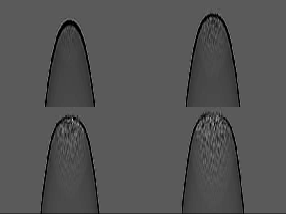
Figure 1. A zoom-in on the wave-field as it propagates into the random boundary. The order in time is top-left, top-right, bottom-left, bottom-right. Note how very little of the wavefront is perturbed at early times.

different
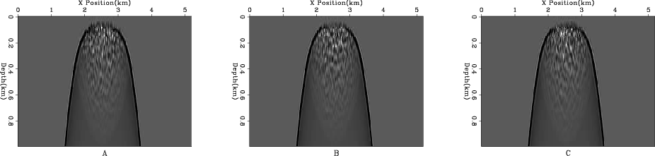
Figure 2. A zoom in on the wave-field as it passes into the random boundary. The three panels represent three different random boundaries. Note the differences in the wave-field leaving the boundary.

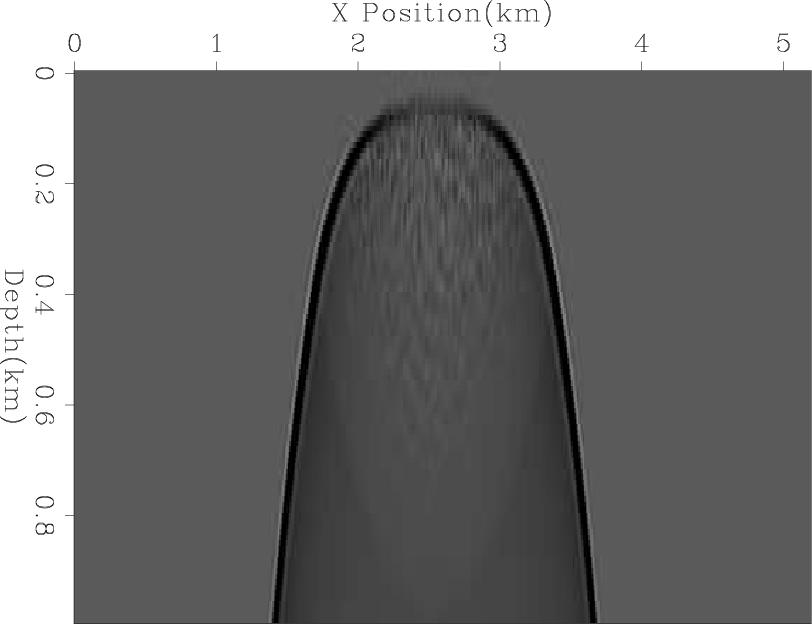
stack1 Figure 3. The result of stacking 16 different random realizations. Note how the noise introduced by the random boundary cancels out when summed.

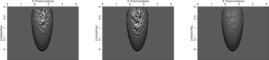
Figures 1-3 are somewhat misleading because the source is in the middle of the computational domain. Figure 4 shows a more realistic scenario where the shot is at the edge of the computational domain. Note the similarity in the wave-fields at early times even with different randomized boundaries. As a result, reflections at these early times (at shallow depths) show many more artifacts than those at later times (Figure 3).

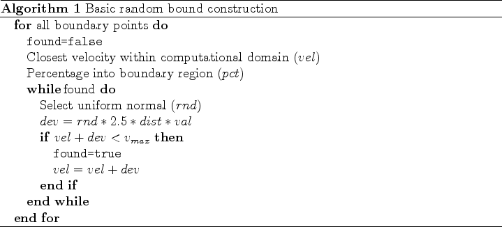
edge
Figure 4. The left and center panels show the wave-field at the same time with two random boundaries generated using algorithm 1. The right panel shows the result of adding 16 realizations together. Note how some energy was stacked coherently.

The shallow depth image can be improved by modifying the random velocity boundary. Algorithm 2 introduces a decreasing maximum velocity towards the outer edge of the computational domain. Energy now takes longer to leave the boundary creating a larger time gap and more random energy pattern between the true wave-field and the noise introduced by the boundary. Figure 5 shows several snapshots with this new boundary condition. Note the increased separation in time and space (compared to the wave-fields seen in Figure 1). The increased time gap and randomness produces less noise at shallow depths (Figure 6).

decrease
Figure 5. The left and center panels show the wave-field at the same time with two random boundaries generated using algorithm 2. The right panel shows the result of adding 16 realizations together. Note how some energy was stacked coherently. Note the larger gap in time between the main wavefront and the energy generated from the random boundary. Further note the decreased energy in the result of stacking multiple realizations.

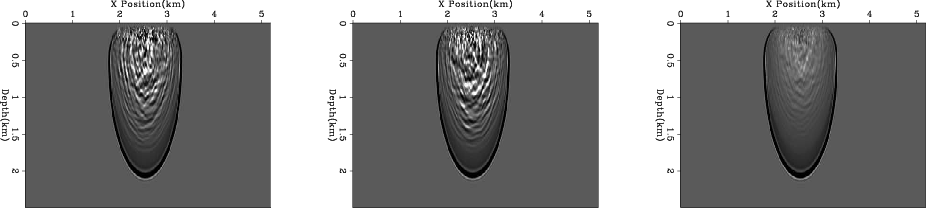
improved
Figure 6. The result of migrating using a damped boundary condition(A), the boundary condition described in algorithm 1 (B), and the boundary condition described in algorithm 2 (C). Note how the shallow reflectors are preserved in (C).

More fun with random boundaries