More fun with random boundaries

VTI random boundaries

Both Clapp (2009) and the previous section describe how to create a boundary for acoustic propagation. VTI propagation is slightly more complicated. We start by defining the horizontal velocity $v_h$ , the vertical velocity $v_v$ , and the the Normal MoveOut velocity $v_{n}$ , defined in terms of Thompson parameters as

$$v_{n} = v_v(1+2 \delta)^{\frac{1}{2}}$$ (1)

and

$$v_{\rm h} = v_v(1+2 \epsilon)^{\frac{1}{2}}.$$ (2)

In acoustic finite difference, a second derivative in x,y, and z ( $p_{d2x},p_{d2y}, p_{d2z}$ ) is calculated at all $ix,iy,$ and $iz$ at a given time step $it$ of the wave-field $p$ . The wave-field at the next time step is then calculated using these derivatives and the sampling in time $dt$ , along with a source term $s$ and the previous value of the wave-field. The computational kernel becomes

$$p(iz,ix,iy,it+1) = p(iz,ix,iy,it+1)-p(iz,ix,iy,it-1)+2p(iz,ix,iy,it)$$

$$+ v(iz,ix,iy)dt^2 (p_{d2x}+p_{d2y}+p_{d2z}).$$ (3)

Following the approach in Alkhalifah (2000) involves an auxiliary wave-field $q$ .; Derivatives in $x$ and $y$ are calculated on $p$ and derivatives in $z$ are calculated on $q$ ($q_{d2z}$ ). The computation kernel then becomes

$$p(iz,ix,iy,it+1) = p(iz,ix,iy,it+1)-p(iz,ix,iy,it-1)+2p(iz,ix,iy,it)$$

$$+ dt^2(v_h(iz,ix,iy)(p_{d2x}+p_{d2y})+v_v(iz,ix,iy)q_{d2z}$$ (4)

and

$$q(iz,ix,iy,it+1) = s(iz,ix,iy,it+1)-q(iz,ix,iy,it-1)+2q(iz,ix,iy,it)$$

$$+ dt^2(v_n(iz,ix,iy)*(p_{d2x}+p_{d2y})+v_v(iz,ix,iy)q_{d2z}.$$ (5)

Randomizing $v_v, v_h,$ and $v_n$ independently creates an unstable system. The most straightforward way to add stable random boundaries to the VTI problem is to create an acoustic random boundary layer by setting $\epsilon$ and $\delta$ to 0 (therefore $v_v=v_h=v_n$ ). A better strategy is to take advantage of the extra flexibility of having three parameters describing moveout. The longer a wavefront travels through the randomized layer, the more chaotic the resulting wave-field and the longer the delay between the true signal and the beginning of noise. By increasing $\epsilon$ and $\delta$ while decreasing $v_v$ we can cause the wave-field to turn parallel to the random boundary. To see this effect, I have removed the random component of the boundary layer while still decreasing $v_v$ and increasing $\epsilon$ and $\delta$ . Figure 7 shows the result of overlaying two wave-fields, one using an isotropic and one using anisotropic boundary. The anisotropic boundary results energy traveling longer in the boundary region. Figure 8 shows the randomized wave-field at several different time steps using both an isotropic and anisotropic boundary condition. Note how the noise pattern using the anisotropic boundary condition is much less regular.

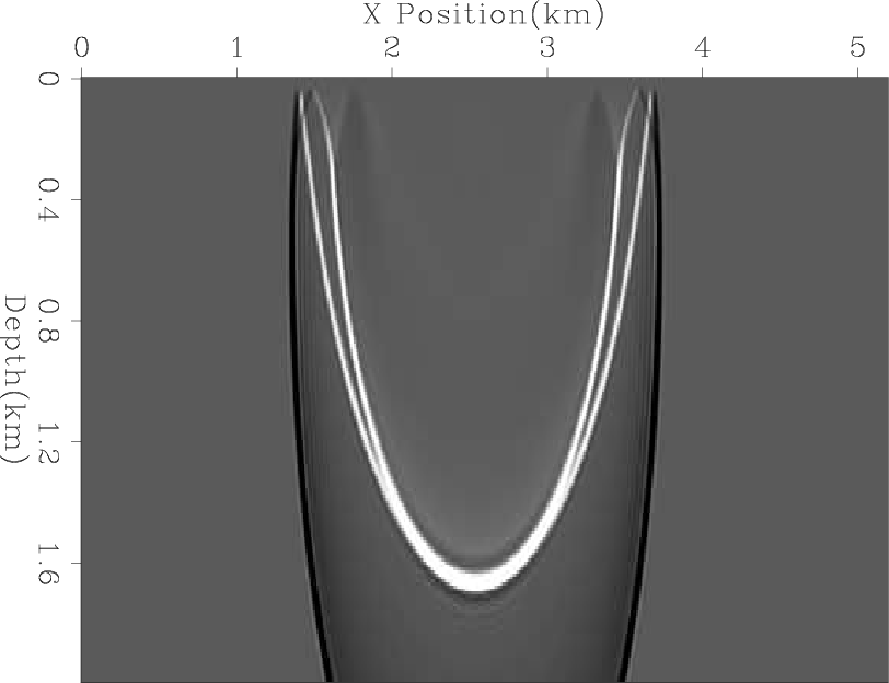
turn Figure 7. The result of overlaying the wave-fields using an isotropic and anisotropic boundary. The anisotropic boundary results in energy traveling longer in the boundary region.

vti
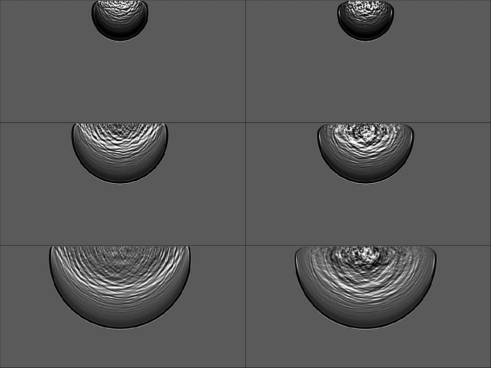
Figure 8. The left panels show a wave-field at several different time steps using an isotropic boundary condition. The right panel shows the wave-field using an anisotropic boundary condition.

More fun with random boundaries