Wave-equation traveltime tomography by global optimization

Theory

The objective function of FWI can be written as follows:

$$\mathbf J_{FWI}(\mathbf v) = \sum_{\mathbf x_s} \sum_{\mathbf x_g... ...athbf x_s;\mathbf v)-\mathbf d_{obs}(t,\mathbf x_g,\mathbf x_s)\vert\vert _2^2,$$ (1)

where $\mathbf x_s$ and $x_r$ are the source and receiver locations, $d_{cal}$ is the modeled data with velocity $\mathbf v$ , and $d_{obs}$ is the observed data. By setting the first derivative of equation (1) around the velocity $\mathbf v_0$ to zero, the velocity update can be expressed as follows:

$$\Delta \mathbf v = \frac{-s}{\mathbf v_0^3}\sum_{\mathbf x_s} \su... ...\mathbf x_g,\mathbf x_s;\mathbf v)-\mathbf d_{obs}(t,\mathbf x_g,\mathbf x_s)),$$ (2)

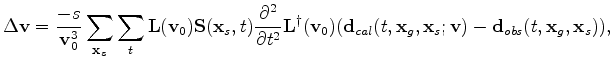where $s$ is the step size, $\mathbf S$ is the source signature, and $\mathbf L$ and $\mathbf L^{\dagger}$ are the forward wave propagation operator and its adjoint, respectively.

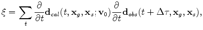
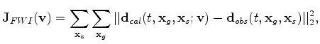
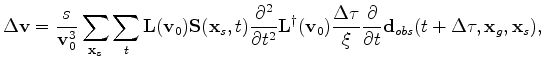
The objective function wave-equation traveltime tomography can be written as follows:

$$\mathbf J_{\Delta \tau}(\mathbf v) = \sum_{\mathbf x_s} \sum_{\mathbf x_g} \vert\vert\Delta \tau(\mathbf x_g,\mathbf x_s;\mathbf v)\vert\vert _2^2,$$ (3)

where $\Delta \tau$ is the lag of the maximum cross-correlation between the observed data and the data modeled by a velocity model $\mathbf v$ . Again, the first derivative of equation (3) around the lags $\Delta \tau$ is set to zero to get the velocity update, which can be expressed as follows:

$$\Delta \mathbf v = \frac{s}{\mathbf v_0^3}\sum_{\mathbf x_s} \sum... ...c{\partial}{\partial t} \mathbf d_{obs}(t+\Delta \tau,\mathbf x_g,\mathbf x_s),$$ (4)

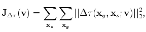
where $\xi$ is defined as follows:

$$\xi = \sum_{t} \frac{\partial}{\partial t} \mathbf d_{cal}(t,\mat... ...c{\partial}{\partial t} \mathbf d_{obs}(t+\Delta \tau,\mathbf x_g,\mathbf x_s),$$ (5)

By examining equations (2) and (4), it can be shown that (WT) can handle much larger velocity errors than (FWI).

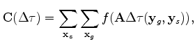
Now, I cast the picking procedure of the lags $\Delta \tau$ as a global optimization problem with an objective function as follows:

$$\mathbf C(\Delta \tau) = \sum_{\mathbf x_s} \sum_{\mathbf x_g} f (\mathbf A \Delta \tau(\mathbf y_g,\mathbf y_s)) ,$$ (6)

where $\mathbf y_g$ and $\mathbf y_s$ are a sparse representation of the source and receiver locations, $\mathbf A$ is a bicubic spline interpolation operator that maps the sparse coordinates $\mathbf y_g$ and $\mathbf y_s$ to the original coordinates $\mathbf x_g$ and $\mathbf x_s$ , and $f$ evaluate the correlation value at $\Delta \tau(\mathbf x_g, \mathbf x_s)$ .

The goal of the global optimization is to maximize the function described by equation (6), which is to maximize the stacking power along the interpolated spline surface. The searching procedure is a simulated annealing algorithm, which varies the spline points along the time axis in a stochastic sense until a satisfying solution is reached. In the following section, I show the results of using such global scheme to pick the correlation lags.

velali
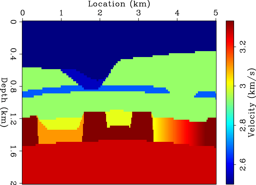
Figure 1. The true velocity model used to create the data.

Wave-equation traveltime tomography by global optimization