Wave-equation traveltime tomography by global optimization

Synthetic example

I use the velocity model shown in Figure 1 to create the synthetic data. The sampling interval of the model is 25 m for both the x-axis and z-axis. The data is modeled using a Ricker wavelet with a fundamental frequency of 15 Hz and a sampling interval of 3 ms. The acquisition geometry is a cross-well configuration, where sources are located in a vertical well on the left side of the model and the receivers are located in a vertical well on the right side of the model. Both the sources and the receivers start at the surface and cover the full depth of the model with a sampling inteval of 25 m.

lags
Figure 2. The correlation lags picked by: (a) the trace-by-trace maximum correlation method, and (b) the global spline-fitting method.

I start the velocity inversion with a constant background velocity of 2.9 km/s, which is very far from the true velocity model. After modeling the data with the background velocity, I cross-correlate the modeled data with the observed data. Figure 2(a) shows the lags picked by maximum correlation at each trace. There is an overall trend from the top left corner to the bottom right corner, which is caused by the gradient in the original data. However, there is also some large anamolies in the picked lags with sharp discontinuities around them. These anomalies are caused by the events refracted by the large velocity contrasts in Figure 1. Figure 2(b) shows the lags picked by the global method, which are significantly different from those in Figure 2(a). The global algorithm ignored the local maximum caused by refracted energy and picked lags that are more consistent with their surroundings.

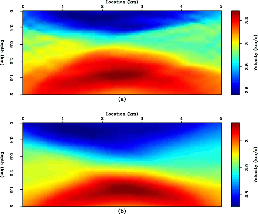
tomo-first
Figure 3. The velocity model after 1 iteration using: (a) the trace-by-trace maximum correlation method, and (b) the global spline-fitting method.

Now, I use the lags estimated by both methods to find a velocity update. The scale of the update is estimated by performing a line search. Figure 3 shows the updated velocity model using both methods after one iteration. The results of the local method shows some noise in the velocity model update, especially around the edges. However, since the velocity update is the sum of the updates of all the shots, the total results are satisfactory. On the other hand, the velocity model estimated by the global method looks cleaner and more consistent laterally. However, the velocity update by the global method shows less detail than that of the local method. In addition, the global method converges at a slower rate than the local method.

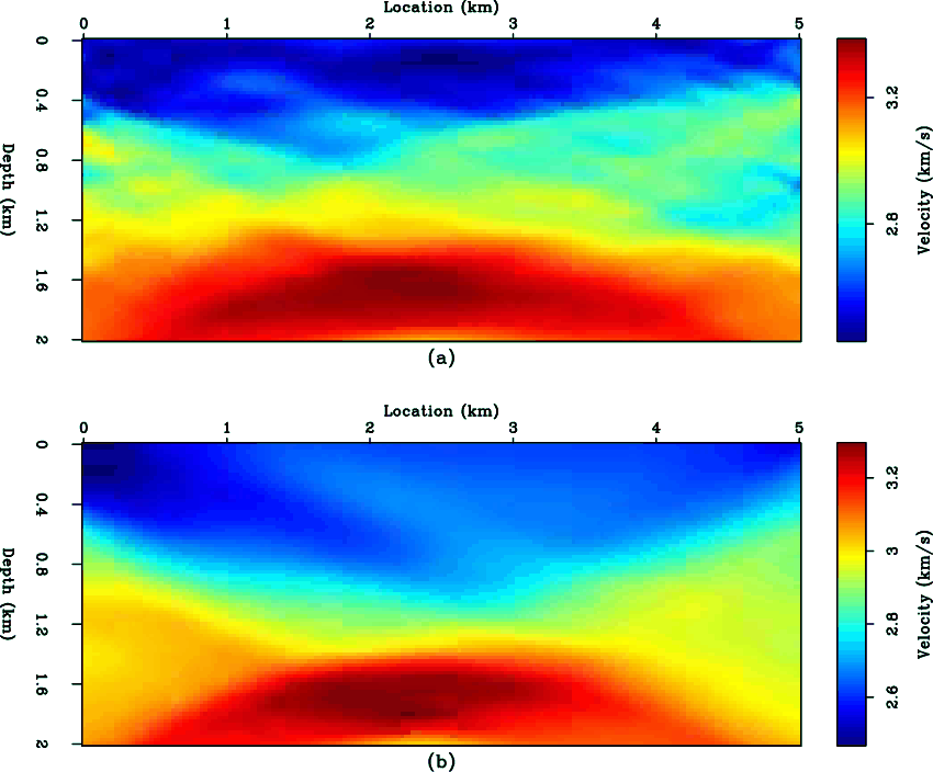
Finally, I run both inversions for 10 iterations to further show the difference between the two methods. The results of both inversions are shown in Figure 4. The noise in the local method estimate grows even larger as I run more iterations, but the accuracy seems to be consistent with the true velocity model. On the other hand, the global method is still too smooth and did not pick the small details as well as the local method. Finally, there seems to be some bias in the global method toward lower velocities.

tomo-last
Figure 4. The inverted velocity model after 10 iterations using: (a) the trace-by-trace maximum correlation, and (b) the global spline-fitting method.

Wave-equation traveltime tomography by global optimization