Geophysical data integration and its application to seismic tomography

Dip residual

In practice, the frequency spectrum of different types of geophysical data can change very widely, and there might be cases with no overlap in frequency band. To address these types of data integration problems, we need to choose properties that are frequency-independent. Local dip is one such property, which can be estimated by solving a regularized optimization (see Fomel (2000) for more details). Given a 2-D field $u(x,z)$, one can estimate the dip values where the data misfit function is given by

$$\begin{cases}\arg \min_{p_u} &  {\bf C}(p_u) {\bf u} \quad \... ...psilon {\bf D} \Delta p_u \thickapprox 0 \ \end{cases} \quad ,$$ (2)

where ${\bf C}(p_u)$ is a convolution operator with a 2-D filter based on the local dip, and ${\bf D}$ represents an appropriate roughening operator. The estimated local dip values are frequency independent, making dip a candidate for carrying geological information from one data field to another. Again, the estimated dips can be used in a regularization term of an optimization problem to impose the structure of the auxiliary data on the estimated model. This model misfit function can be given as follows:

$$r_m(x,z)=(\frac{\partial}{\partial x}+p_u \frac{\partial}{\partial z}) v(x,z) \thickapprox 0.$$ (3)

Note that the structural similarity measures do not include any physical link that might potentially exist between two fields. In other words, these functions only help the model-shaping part of optimization, and the physics of estimation lies in the data-misfit term with the mapping operator.

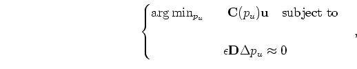
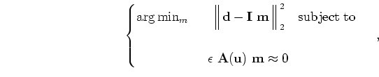
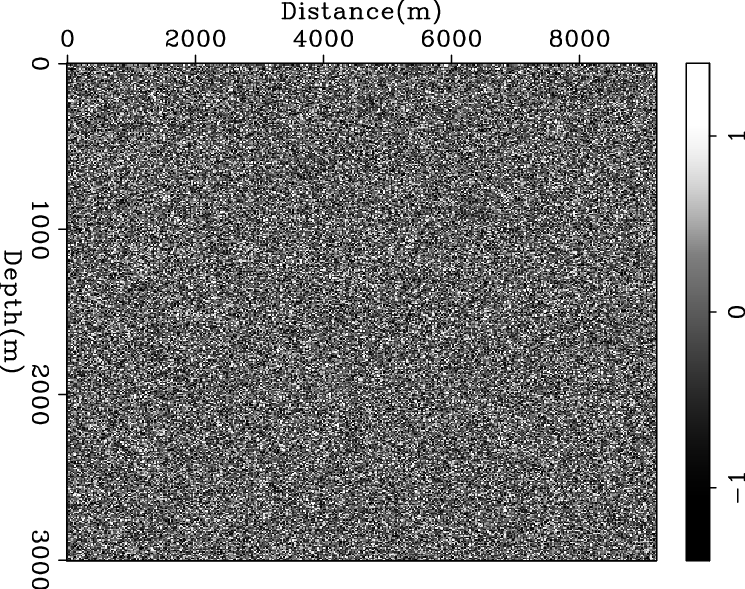
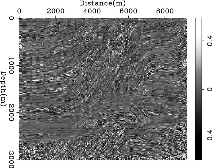
Figures 1 and 2 show examples where the reflectivity of the Marmousi synthetic model is used as auxiliary data to impose the geophysical structures on a random noise field and a smooth velocity field. The optimization problem used to generate the estimated model shown by Figures 1 and 2 is given by

$$\begin{cases}\arg \min_{m} &  \Big \Arrowvert {\bf d} - {\bf... ...{\bf A}({\bf u}) {\bf m} \thickapprox 0 \ \end{cases} \quad ,$$ (4)

where ${\bf I}$ is identity matrix; ${\bf A}$ is either the cross-gradient or dip residual operator; ${\bf u}$ and ${\bf d}$ represent the auxiliary reflectivity field and the data (noise or smooth velocity field), respectively; and ${\bf m}$ is the estimated model which incorporates some of the structural information provided by ${\bf u}$. Note that a large $\epsilon$ is needed to emphasize on model-shaping term and impose structure. Figures 1(a) and 2(b) show the data ${\bf d}$ and the auxiliary field ${\bf u}$. Figure 1(d) shows a better reconstruction of the Marmousi structure with dip residual technique than the cross-gradient function (Figure 1(c)). This is clearly visible by comparing the continuity of reconstructed amplitude along the geological dips in Figure 1(d)).

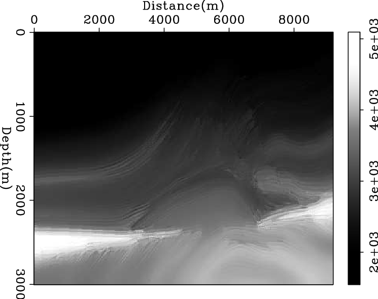
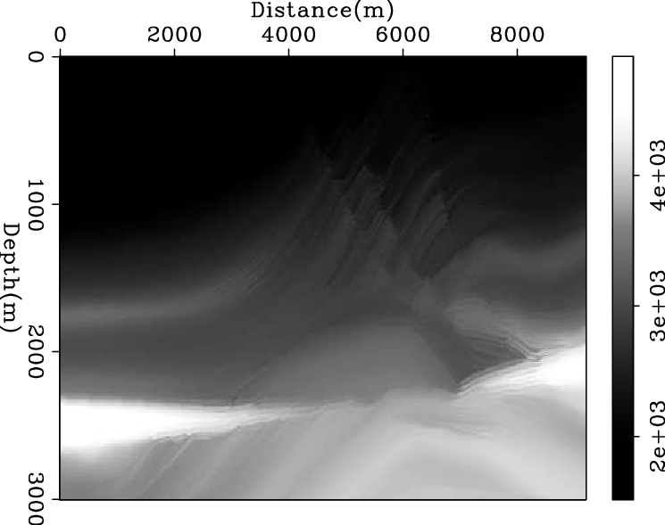
Figure 2 shows a similar problem where we start with a smooth velocity of the Marmousi model instead of noise. Similarly, Figure 2(d) suggests that the dip residual technique leads to a less noisy partial reconstruction of the Marmousi structure; but not all the details are included. However, some of the horizontal parts of structures are reconstructed by the cross-gradient function (Figure 2(c)), but not with the dip residual (Figure 2(d)). Note that frequency ranges in smooth velocity and reflectivity are low and high, respectively.

noise,ref,nxrx,nxrp
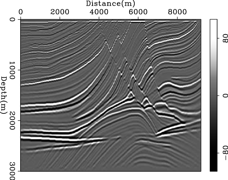
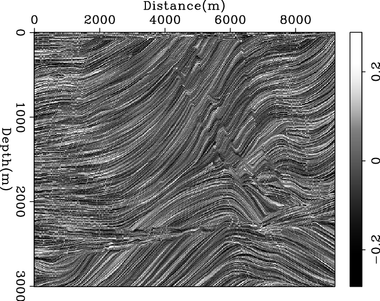
Figure 1. Data integration problem 1: The starting model is random noise (a) and the auxiliary data is the reflectivity of the Marmousi model (b). Panel (c) shows the estimated model with the cross-gradient function and panel (d) shows the estimated model with the dip residual. Note the reconstruction of the structure in the estimated models and how each method provides different quality of reconstruction. [ER]

vs,ref,mxrx,mxrp
Figure 2. Data integration problem 2: The starting model is now changed to a smooth version of velocity (a) and the auxiliary data is the reflectivity of the Marmousi model (b) . Next panels show the estimated model with (c) the cross-gradient function and (d) dip residual. Note that we only expect to reconstruct the structure of the model, and the formulation of our optimization problems does not include the physics behind the wave propagation. [ER]

Geophysical data integration and its application to seismic tomography