Applications of the generalized norm solver

Formulation of the 1D Galilee Problem

Our next test case is the removal of spikes and drift from a 1-dimensional representation of the Galilee depth data. We constructed this experiment to be more rigorous than the earlier line-fitting and noise-removal problem. The 1D Galilee problem is a synthetic problem that originates from a depth sounding experiment on the Sea of Galilee. Imagine performing a depth-sounding experiment along a fixed track in the lake. The lake has a sinusoidal depth with blocky drift and large spikes in time. As a boat goes back and forth across this 1D lake, it is measuring the sum of the true lake depth plus the drift in time. Figure 2 shows the true depth of our 1D Galilee lake and figure 3 shows the recorded data, which is the sum of the drift function and the true depth. We have added 2 spikes as outliers in the data. These 2 spikes can be viewed as equipment failure. Note that the data covers the lake back and forth roughly 6.25 times.

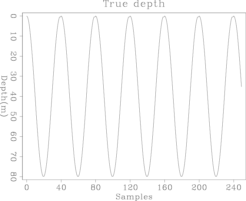
truedepth Figure 2. The true depth of the Sea of Galilee along a fixed track. [ER]

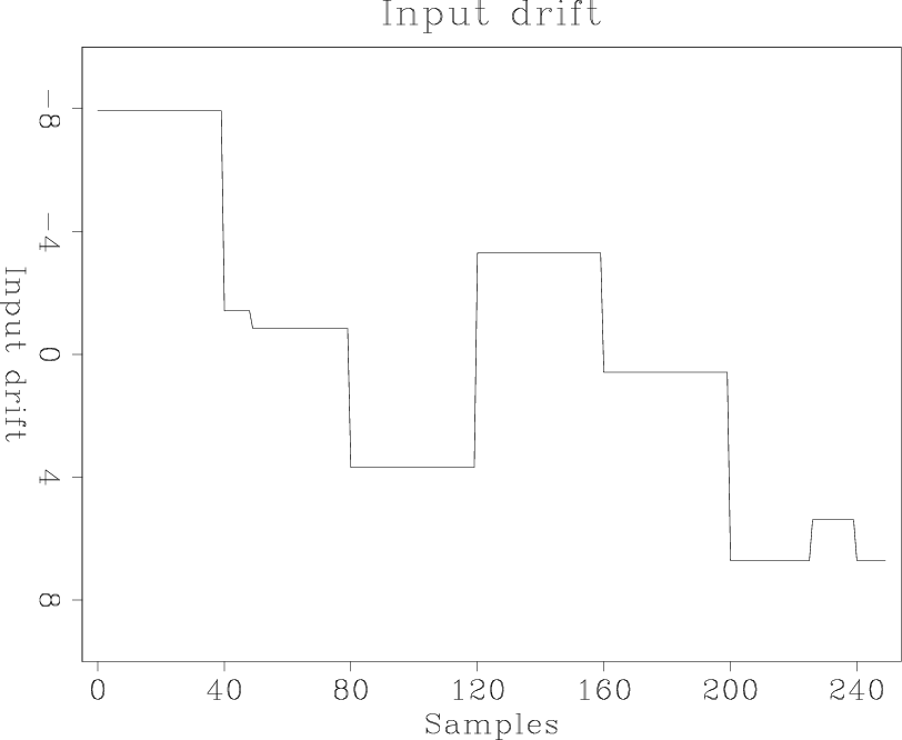
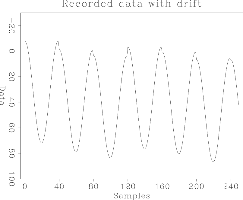
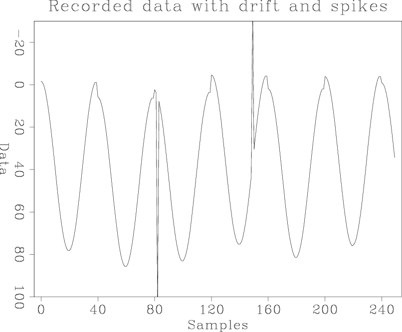
data-drift,data-aq1,data-aq2
Figure 3. (a) The drift as a function of aquisition time. (b) The recorded data, which is the sum of the true lake depth and drift. (c) The recorded data with two outliers. The two spikes are added to the data to account for equipment failure.[ER]

To formulate the problem for inversion, we have set our unknown model space to be the lake depth, $\bold m$, and the drift function, $\bold u$. Data space $\bold d$ is the recorded depth as shown in Figure 3. Our data fitting goal can be defined as

$$0 \approx \bold L \bold m + \bold u - \bold d,$$ (3)

where $\bold L$ is the binning operator that matches the data acqusition in time to its corresponding location in space. For a lake with 4 grid points and 6 data points, equation 3 would look like this:

$$0 \approx \left[ \begin{array}{cccc} 1 & 0 & 0 & 0 \\ 0 & 1 & 0 ... ...[ \begin{array}{c} d_1 \ d_2 \ d_3 \ d_4 \ d_5 \ d_6 \end{array} \right].$$

Equation 3 by itself is an under-determined problem, because there are more unknowns than the recorded data points. If there are 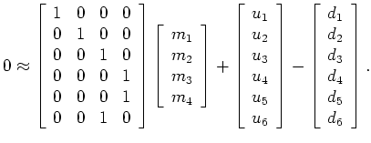$n_d$ data points and the lake has $n_m$ grid points, then the model space has a dimension of $n_m + n_d$, because we are solving for both lake depth and drift in time. The data space has a dimension of $n_d$. To introduce more constraints, we can add a regularization by requiring the drift function $\bold u$ to be smooth,

$$0 \approx \frac{d}{dt} \bold u .$$ (4)

It is worth pointing we only expect good results when we run this regularization with $L1$ or $L1$-type norms, as $L2$ smoothing will wipe out the ``blockiness" in the drift function, which is part of the model space. To illustrate the limitation of least-squares fitting, I will first show the result of applying inversion to the 1D Galilee problem.

Applications of the generalized norm solver