|
|
|
|
Schoenberg's angle on fractures and anisotropy: A study in orthotropy |
For waves propagating in the [![]() -
-![]() ]-plane with wavenumbers
]-plane with wavenumbers
![]() and
and
![]() where
where
![]() ,
Tsvankin (1997) shows that we have the following equations
[patterned here after the notation of Berryman (1979)]:
,
Tsvankin (1997) shows that we have the following equations
[patterned here after the notation of Berryman (1979)]:
Sayers and Kachanov (1991) consider a model with two sets of possibly nonorthogonal
fractures, also possibly having two different fracture density values
![]() and
and ![]() . Total fracture density is therefore
. Total fracture density is therefore
![]() .
These authors found that the pertinent fracture influence parameters were multiplied
in this situation, when the angle between the fracture sets is
.
These authors found that the pertinent fracture influence parameters were multiplied
in this situation, when the angle between the fracture sets is ![]() ,
either solely by
,
either solely by ![]() itself or by one of the two factors:
itself or by one of the two factors:
Table 1 shows the Sayers and Kachanov (1991) results for corrections
to the isotropic background values of compliance (in Voigt 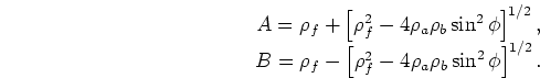 matrix notation -- the original paper had results expressed
in terms of tensor notation). Those background values
are specfically for one model considered having Poisson's ratio
matrix notation -- the original paper had results expressed
in terms of tensor notation). Those background values
are specfically for one model considered having Poisson's ratio
![]() (dimensionless), effective bulk modulus
(dimensionless), effective bulk modulus ![]() ,
shear modulus
,
shear modulus ![]() , and Young's modulus
, and Young's modulus ![]() ,
with all moduli measured in units of GPa.
For the assumed inertial density
,
with all moduli measured in units of GPa.
For the assumed inertial density ![]() kg/m
kg/m![]() , the
resulting isotropic background compressional wave speed is
, the
resulting isotropic background compressional wave speed is ![]() km/s
and shear wave speed is
km/s
and shear wave speed is ![]() km/s.
For our computations, we also need the isotropic background compliance
values, which are
km/s.
For our computations, we also need the isotropic background compliance
values, which are
![]() ,
,
![]() , and
, and
![]() . The fracture influence factors
. The fracture influence factors ![]() and
and ![]() , found
for this specific model by Berryman and Grechka (2006), are displayed in
Table 2.
Some higher order fracture-influence factors were also obtained
in the earlier work, but I will not be considering such factors
in this short paper.
, found
for this specific model by Berryman and Grechka (2006), are displayed in
Table 2.
Some higher order fracture-influence factors were also obtained
in the earlier work, but I will not be considering such factors
in this short paper.
|
|
||
|
|
||
In the examples that follow, I will consider only the case of equal
fracture densities
![]() . For this somewhat
simpler situation, I also have
. For this somewhat
simpler situation, I also have
| Fracture parameter | GPa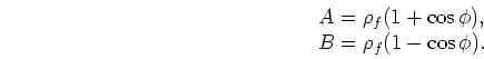 |
| |
There may also be some uncertainty about exactly which of these factors is
which in this degenerate case, because of the sign ambiguity in taking
the square root of ![]() . But I will not concern myself with this detail here.
. But I will not concern myself with this detail here.
|
|
|
|
Schoenberg's angle on fractures and anisotropy: A study in orthotropy |