|
|
|
|
Gradient of image-space wave-equation tomography by the adjoint-state method |
 and 16 m in
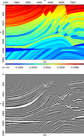
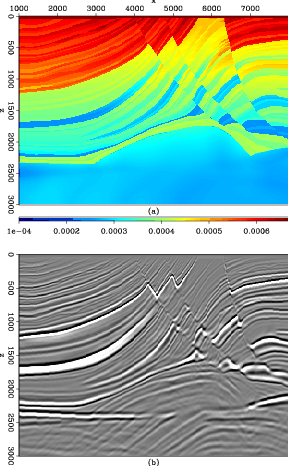
 The one-way shot profile image with the correct slowness model can be seen in Figure 1b. The modeled data were also migrated using the background slowness of Figure 2a to compute the background image of Figure 2b. The background slowness differs from the true slowness in a limited region, as can be seen in Figure 3, which shows the ratio between true and background slowness. When comparing the two images, there is a clear pull-up effect at the center-bottom of the background image caused by migrating with a velocity which is too slow.
|
|---|
|
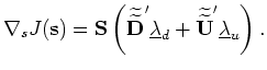
true
Figure 1. (a) True slowness of the Marmousi model. (b) Zero-subsurface-offset section of the one-way shot-profile migration with the true slowness model.[CR] |
|
|
|
|---|
|
bckg
Figure 2. (a) Background slowness. (b) Zero-subsurface-offset section of the one-way shot-profile migration with the background slowness model.[CR] |
|
|
|
|---|
|
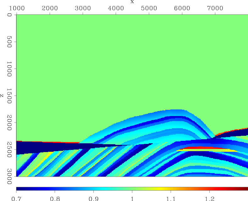
dslow
Figure 3. Ratio between the true and the background slowness.[ER] |
|
|
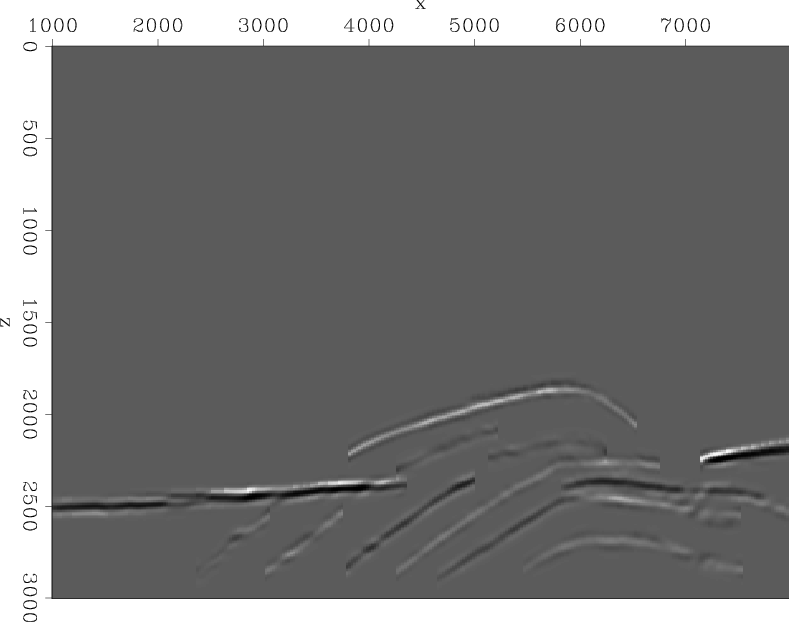
Following Guerra et al. (2009), representative reflectors were selected from the background image (Figure 4) to synthesize eleven image-space phase-encoded source and receiver wavefields using the background slowness. Prior to modeling, the selected reflectors were subjected to rotation according to the apparent geological dip as previously mentioned. I estimate that, by using only eleven areal shots, the computational cost decreased in ![]() considering if the slowness optimization was carried out with the original 376 shot-profiles.
considering if the slowness optimization was carried out with the original 376 shot-profiles.
|
|---|
|
bwkim
Figure 4. Zero-subsurface-offset section showing the reflectors selected on the one-way shot-profile migration with the background slowness model.[CR] |
|
|
The optimization stopped after 4 iterations comprising 41 function and gradient evaluations. The optimized slowness model can be seen in Figure 5a. The optimized slowness decreased as expected, but did not recover the details of the true slowness. The smoothness of the optimized slowness is partially because of the B-spline filtering of the gradient but also because image-space wave-equation tomography cannot solve for the short wavelengths of the slowness model, as pointed out by Symes (2008).
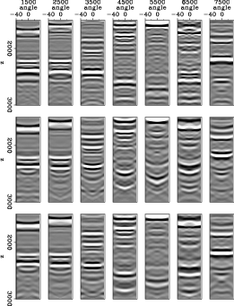
The accuracy of the optimized slowness model can be evaluated by comparing the computed images with true, background, and optimized slowness. The shot-profile migration of the original shots using the optimized slowness is shown in Figure 5b. Notice that the pull-up effect, which occurs in the background image, is greatly mitigated. In addition, reflectors are more focused in the image computed with the optimized slowness than in the image computed with the background slowness. Another slowness accuracy indicator is flatness of the reflectors in the ADCIGs. The ADCIGs resulting from shot-profile migration of the original shots using, from top to bottom, the true slowness, the background slowness and the optimized slowness are shown in Figure 6. The reflectors computed with the optimized slowness are flatter than those with the background slowness, demonstrating the greater accuracy of the optimized slowness.
|
|---|
|
opti
Figure 5. (a) Optimized slowness after 4 iterations with 41 function and gradient evaluations. (b) Zero-subsurface offset section of the one-way shot-profile migration with the optimized slowness model.[CR] |
|
|
|
|---|
|
fang1
Figure 6. ADCIGs obtained with true slowness (top), background slowness (center), and optimized slowness (bottom).[CR] |
|
|
|
|
|
|
Gradient of image-space wave-equation tomography by the adjoint-state method |