|
|
|
|
Gradient of image-space wave-equation tomography by the adjoint-state method |
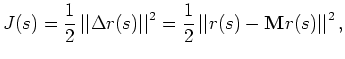 is the image perturbation that measures the accuracy of the slowness model. To compute
If the differential residual-focusing operator ![]() is independent of the slowness, the gradient of this objective function evaluated at the current slowness
is independent of the slowness, the gradient of this objective function evaluated at the current slowness
![]() is
is
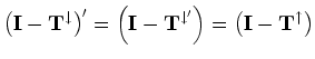
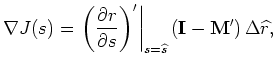 is the identity operator, and
Because the image-space wave-equation tomographic operator is composed of different operators, it is difficult to envision from equation 8 which operations are performed to compute the gradient. Therefore, for a clear explanation of the operators involved, I use the adjoint-state method to derive the gradient of the objective function (equation 7).
In migration with generalized sources or shot-profile migration, the source and receiver wavefields are propagated independently, and the image
![]() at a depth level
at a depth level ![]() , is computed by the crosscorrelation
, is computed by the crosscorrelation
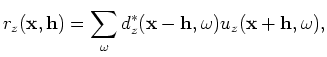 is the source wavefield for a single frequency
In a more compact notation, not explicitly writing the dependencies on ![]() and
and ![]() , equation 9 can be re-written as follows:
, equation 9 can be re-written as follows:
and
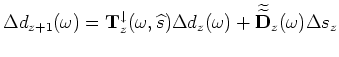
For subsequent depth levels,
![]() is computed by means of the recursive downward propagation
is computed by means of the recursive downward propagation
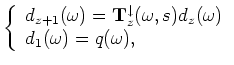 is the downward continuation operator, which is a function of the slowness
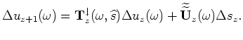
The downward continuation of the receiver wavefield is performed by
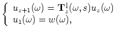 is the recorded data at the surface for shot-profile migration. If using generalized sources in the image space, is the phase-encoded areal receiver wavefield of equation 4. In equations 11 and 12, I omitted the dependencies of the wavefield with respect to
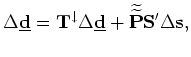
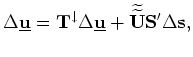
In the image-space wave-equation tomography problem, the perturbed source and receiver wavefields, and the image perturbation are used to compute the slowness perturbation that updates the current slowness model. From the perturbation theory, we have
![]() ,
,
![]() , and, consequently,
, and, consequently,
![]() are physical realizations with
are physical realizations with
![]() , where the
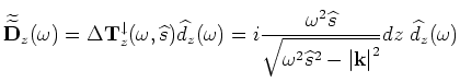
, where the ![]() refers to fields obtained with the background slowness. To the first order (Born approximation), these perturbed fields are given by
refers to fields obtained with the background slowness. To the first order (Born approximation), these perturbed fields are given by
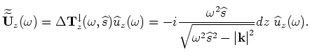
 and
and
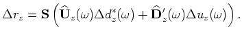
The perturbed image is given by
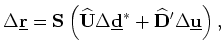 is a spreading operator that replicates the slowness perturbation for every frequency.
Equations 18, 19, and 20 are the forward modeling equations of the image-space wave-equation tomography problem using the generalized sources or shot-profile schemes. They depend on the state variables
![]() ,
,
![]() , and
, and
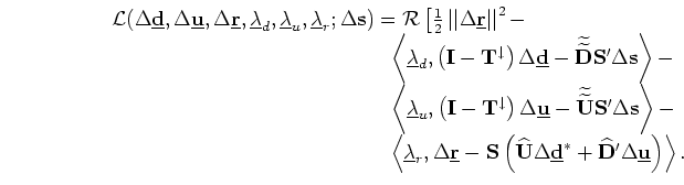
![]() . Plessix (2006) describes how to compute the adjoint states using the augmented functional methodology. By introducing the adjoint-state variables
. Plessix (2006) describes how to compute the adjoint states using the augmented functional methodology. By introducing the adjoint-state variables
![]() ,
,
![]() , and
, and
![]() , the augmented Lagrangian reads
, the augmented Lagrangian reads
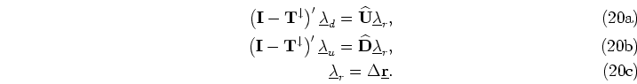
 with respect to the state variables and equating to zero, which gives
 |
(22) |
Finally, the gradient of  is
is
|
|
|
|
Gradient of image-space wave-equation tomography by the adjoint-state method |