Selecting the right hardware for Reverse Time Migration

Following the wavefield

The computational domain used for RTM is usually controlled by the desired migration aperture. The source function $w$ from algorithm 2 is non-zero in a very small portion of the computational domain. When propagating a source, we might have as few as 9 non-zero elements in a mesh that is a billion points in size. As a result, at early times, algorithm 2 would spend over 99% of its efforts propagating zeros. As time progresses, the wavefield will be non-zero at a larger percentage of the volume. As Figure 1 shows, we can slowly expand the range of $ix,iy$ and $iz$, reducing the total number of operations.

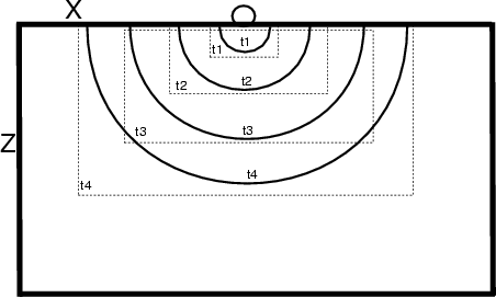
range Figure 1. An illustion of how we can restrict the size of computational domain at early times. The circle represents a source at the surface and the wavefronts are drawn different time locations (t1,t2,t3). The domain where we update our wavefield can safely be restricted to the corresponding boxes.[NR]

Selecting the right hardware for Reverse Time Migration