Selecting the right hardware for Reverse Time Migration

RTM

The concept behind RTM is relatively simple. We start with a known earth model. This earth model might be simply acoustic velocity but can be anisotropic, elastic, or even visco-elastic. Two different modeling experiments are conducted simultaneously through the earth model. Both attempt to simulate the seismic experiment conducted in the field, one from the perspective of the source and one from the perspective of the receivers. The source experiment involves injecting our estimated source wavelet into the earth and propagating it from $t=0$ to our maximum recording time $t_{\rm max}$, creating a 4-D source field $s(x,y,z,t)$. At the same time, we conduct the receiver experiment. We inject and propagate our recorded data starting from $t_{\rm max}$ to $t_0$, creating a similar four dimensional volume $g(x,y,z,t)$. The most common approach is to propagate these fields using an explicit time marching scheme (Dablain, 1986). We start from the acoustic wave equation

$$\frac{\partial ^2 u}{\partial t^2} = \bf v^2 \left( \frac{\p... ...^2 }{\partial y^2} + \frac{\partial^2 }{\partial z^2} \right),$$ (1)

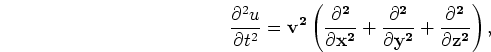where $u$ is pressure and $\bf v$ is velocity. We can use a Taylor expansion to approximate these derivatives. Algorithm 2 shows the pseudo-code for how to forward propagate by $nt$ steps a source function $w$, with a $dt$ interval on a regular mesh whose size is $nx,ny,nz$ indexed by $ix,iy,iz,it$, using a second-order approximation of the time and space derivatives.

We have a reflection where the energy propagated from the source and the receiver are located at the same position at the same time. The final image 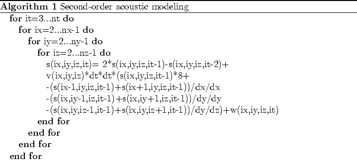$i$ is the summation of correlating the source and receiver wavefield at every time and every shot,

$$i(x,y,z)=\sum_{\rm shots}\sum_{t=0}^{t_{\rm max}} s(g,x,y,z,t) g(x,y,z,t).$$ (2)

Selecting the right hardware for Reverse Time Migration