|
|
|
|
Least-squares migration/inversion of blended data |
| (6) |
The advantage of the model-space formulation is that it can be implemented in a target-oriented fashion, which can substantially reduce the size
of the problem and hence the computational cost (Valenciano, 2008).
However, it requires explicitly computing the Hessian operator, which is expensive without certain approximations.
As demonstrated by Valenciano (2008),
for a typical conventional acquisition geometry, i.e., when
![]() , the Hessian operator
, the Hessian operator
![]() is diagonally dominant
for areas of good illumination, but for areas of poor illumination, the diagonal energy spreads along its off-diagonals.
The spreading is limited and can almost be captured by a limited number of off-diagonal elements. That is why Valenciano (2008)
suggests computing a truncated Hessian filter to approximate the exact Hessian for inverse filtering.
Doing this makes the cost of the model-space inversion scheme affordable for practical applications.
Figure 8(a) shows the local Hessian operator located at
is diagonally dominant
for areas of good illumination, but for areas of poor illumination, the diagonal energy spreads along its off-diagonals.
The spreading is limited and can almost be captured by a limited number of off-diagonal elements. That is why Valenciano (2008)
suggests computing a truncated Hessian filter to approximate the exact Hessian for inverse filtering.
Doing this makes the cost of the model-space inversion scheme affordable for practical applications.
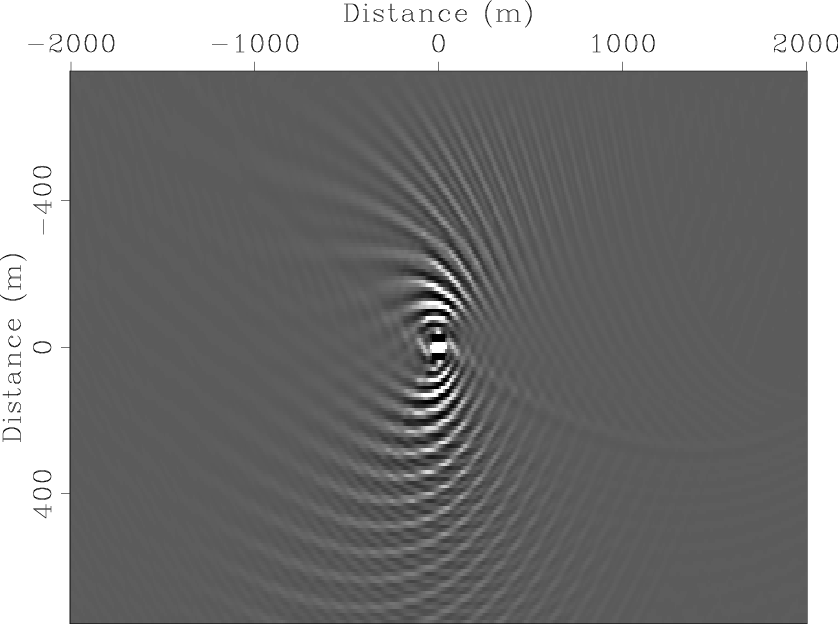
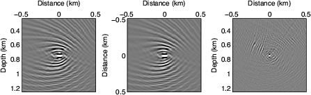
Figure 8(a) shows the local Hessian operator located at ![]() m and
m and ![]() m in the subsurface
(a row of the entire Hessian matrix) for the previous scattering model with
the conventional acquisition geometry. The origin of this plot denotes the diagonal element of the Hessian,
while locations not at the origin denote the off-diagonal elements of the Hessian.
As expected, the Hessian is well focused around its diagonal part, and hence can be approximated by a filter with a small size.
However, for the blended acquisition geometry, the combined modeling operator
m in the subsurface
(a row of the entire Hessian matrix) for the previous scattering model with
the conventional acquisition geometry. The origin of this plot denotes the diagonal element of the Hessian,
while locations not at the origin denote the off-diagonal elements of the Hessian.
As expected, the Hessian is well focused around its diagonal part, and hence can be approximated by a filter with a small size.
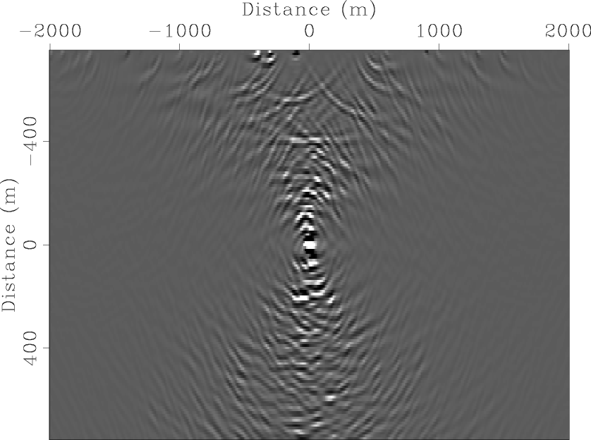
However, for the blended acquisition geometry, the combined modeling operator
![]() becomes far from unitary, and hence the Hessian
becomes far from unitary, and hence the Hessian
![]() has non-negligible off-diagonal energy,
which can spread over many of the off-diagonal elements. This phenomenon is confirmed by
Figure 8(b) and Figure 8(c), which show the local Hessian operators at the same
image point for different blended acquisition geometries. It is clear that a filter with a small size could
not capture all the important characteristics of the crosstalk in the migrated image; therefore
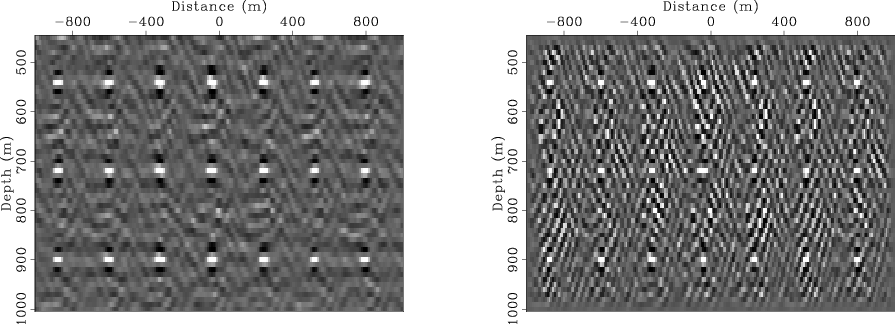
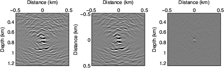
inverse filtering would fail to remove the crosstalk. Figure 9 shows
the model-space inversion result with a small Hessian filter (
has non-negligible off-diagonal energy,
which can spread over many of the off-diagonal elements. This phenomenon is confirmed by
Figure 8(b) and Figure 8(c), which show the local Hessian operators at the same
image point for different blended acquisition geometries. It is clear that a filter with a small size could
not capture all the important characteristics of the crosstalk in the migrated image; therefore
inverse filtering would fail to remove the crosstalk. Figure 9 shows
the model-space inversion result with a small Hessian filter (
![]() in size) for both blended acquisition geometries.
The crosstalk is not removed at all, and the inverted images become even worse.
in size) for both blended acquisition geometries.
The crosstalk is not removed at all, and the inverted images become even worse.
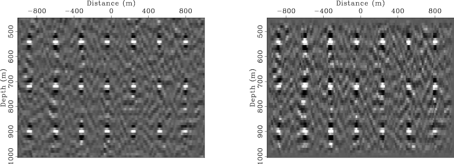
For comparison, Figure 10 shows the inversion result with the full Hessian for a model with only one scatterer in the subsurface (the blending parameters are the same as those for the multiple scattering model). The full Hessian includes all possible off-diagonal elements, so it accurately predicts the crosstalk pattern. The inversion successfully removes the crosstalk. However, the full Hessian is too expensive to compute even though it is target-oriented, and the cost of computing many off-diagonals can quickly outweight the achieved savings of performing the inversion in a target-oriented fashion. Therefore, we seek an inversion approach that does not require explicitly computing the Hessian, so that we do not have to worry about the size of the Hessian filter. This important consideration leads us to the following data-space inversion approach.

|
|---|
|
pts-hess-super-shtpro,pts-hess-super-planes-2,pts-hess-super-randts
Figure 8. The local Hessian operator located at |
|
|
|
|---|
|
pts-imag-invt-planes-2,pts-imag-invt-randts
Figure 9. Comparison between migration and model-space LSI with a small Hessian ( |
|
|
|
|---|
|
pts-single-decon-planes-2,pts-single-decon-randts
Figure 10. Comparison between migration and model-space LSI with a full Hessian ( |
|
|
|
|
|
|
Least-squares migration/inversion of blended data |