|
|
|
|
Least-squares migration/inversion of blended data |
There are many choices of the blending operator; which one produces the optimal imaging result might be case-dependent and is beyond the scope of this paper.
In this paper, we mainly consider two different blending operators: a linear-time-delay blending operator and a random-time-delay blending operator.
The first operator seems to be common and
easy to implement in practice for acquiring marine data,
while the second one is interesting and has been partially adopted in acquiring both land and marine data with
simultaneous shooting (Hampson et al., 2008). For example,
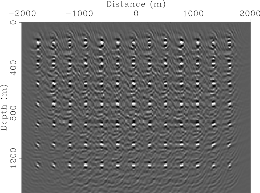
Figure 1 shows a scattering reflectivity model with a constant velocity of ![]() m/s.
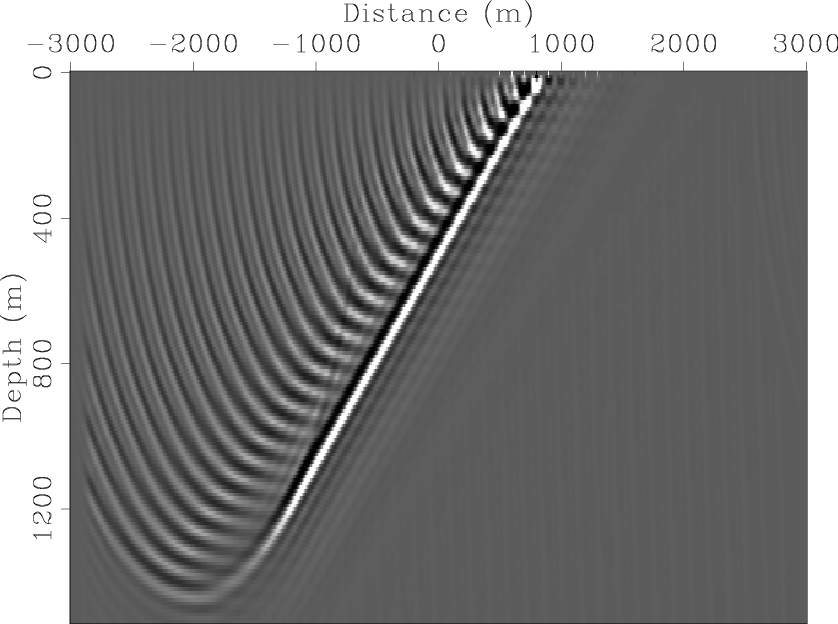
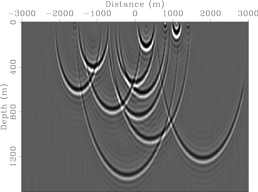
Figure 2 and
Figure 3 show the snapshots of the corresponding blended source wavefields.
For both cases,
m/s.
Figure 2 and
Figure 3 show the snapshots of the corresponding blended source wavefields.
For both cases, ![]() point sources with an equal spacing of
point sources with an equal spacing of ![]() m are blended into one composite source.
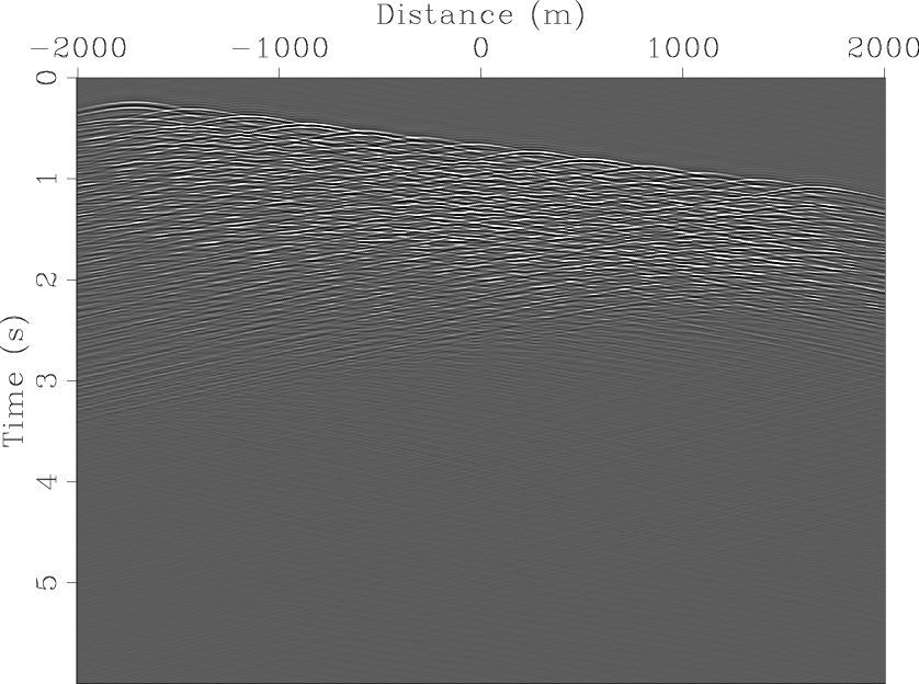
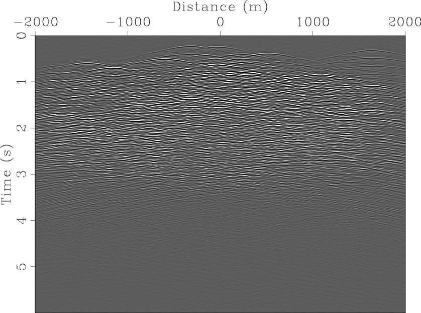
Figure 4 shows the modeled blended data.
Given the complexity of the super-areal shot gathers shown in Figure 4,
it might be very difficult or even impossible to deblend them.
m are blended into one composite source.
Figure 4 shows the modeled blended data.
Given the complexity of the super-areal shot gathers shown in Figure 4,
it might be very difficult or even impossible to deblend them.

|
|---|
|
pts-refl
Figure 1. A reflectivity model containing many point scatterers. [ER] |
|
|
|
|---|
|
pts-wfds-planes-2
Figure 2. Source wavefield after linear-time-delay blending. [CR] |
|
|
|
|---|
|
pts-wfds-randts
Figure 3. Source wavefield after random-time-delay blending. [CR] |
|
|
|
|---|
|
pts-trec-planes-2,pts-trec-randts
Figure 4. Modeled blended shot gather. (a) Linear-time delay blending and (b) random-time-delay blending. [CR] |
|
|
We can directly use the adjoint of the combined modeling operator, which is also widely known as the migration operator,
to reconstruct the reflectivity as follows:
|
|---|
|
pts-mig-planes-2
Figure 5. Migration of linear-time-delay blended data. [CR] |
|
|

|
|---|
|
pts-mig-randts
Figure 6. Migration of random-time-delay blended data. [CR] |
|
|

|
|---|
|
pts-mig-shtpro
Figure 7. Migration of the data acquired with the conventional acquisition geometry. [CR] |
|
|
|
|
|
|
Least-squares migration/inversion of blended data |