|
|
|
|
Inversion of up and down going signal for ocean bottom data |
The inverse problem for imaging multiples using up- and down-going data can be fomulated as follow.
We first break down the recorded data as the superposition of up-
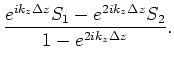 and down-going
![]() signals at the receivers. This can be done by using PZ data to give up-going and down-going data as discussed in the PZ summation section above.
signals at the receivers. This can be done by using PZ data to give up-going and down-going data as discussed in the PZ summation section above.
The above construction assumes that the vertical particle velocity 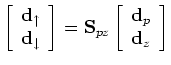 contains mostly pressure (
![]() ) waves. A pre-processing step can be included into
) waves. A pre-processing step can be included into
![]() to separate the
to separate the ![]() and converted
and converted ![]() wave arrivals (Helbig and Mesdag, 1982; Dankbaar, 1985). Next, we denote the modelling operator for up-going signals at the receivers as
wave arrivals (Helbig and Mesdag, 1982; Dankbaar, 1985). Next, we denote the modelling operator for up-going signals at the receivers as
![]() . Similarily, denote the modeling operator for down-going signals at the receivers as
. Similarily, denote the modeling operator for down-going signals at the receivers as
![]() . The two modeling operators provide the up- and down-going modeled data, denoted as
. The two modeling operators provide the up- and down-going modeled data, denoted as
![]() and
and
![]() ;
;
The inverse problem is defined as minimizing the ![]() norm of the two data residuals
norm of the two data residuals
![]() and
and
![]() , with respect to a single model
, with respect to a single model ![]() . The data residuals are defined as the difference between the recorded data and the modelled data,
. The data residuals are defined as the difference between the recorded data and the modelled data,
where
![]() represents the
represents the ![]() norm. In matrix form, the fitting goal can be written as
norm. In matrix form, the fitting goal can be written as
With the conjugate gradient method, the model update
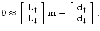 at each iteration has contributions from both the up-going and down-going parts of the inversion;
where
![]() and
and
![]() is the up- and down-going part of the residual, respectively.
is the up- and down-going part of the residual, respectively.
The justification for this inverse problem is to reduce the wrong placement of image point with the use of both
and
![]() signals. Traditional migration scheme only uses
signals. Traditional migration scheme only uses
![]() to determine the image since all primary signal can be found in
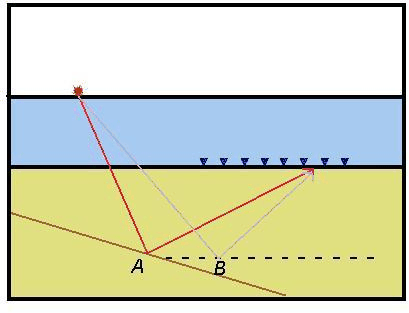
. However, migration of primaries can give incorrect image point as well. In Figure 4, a primary event with a given travel time can indicate a correct image point at A and an incorrect image point at B. If we include the previously ignored information
to determine the image since all primary signal can be found in
. However, migration of primaries can give incorrect image point as well. In Figure 4, a primary event with a given travel time can indicate a correct image point at A and an incorrect image point at B. If we include the previously ignored information
![]() into a joint inversion, some wrongly placed image point can be refuted. Joint imaging allow us to use both primaries and multiples to estimate the image. This can be a distinct advantage because multiples and primaries illuminate different parts of the sub-surface. For ocean bottom data with sparse receiver spacing, multiples illuminate more than primaries.
into a joint inversion, some wrongly placed image point can be refuted. Joint imaging allow us to use both primaries and multiples to estimate the image. This can be a distinct advantage because multiples and primaries illuminate different parts of the sub-surface. For ocean bottom data with sparse receiver spacing, multiples illuminate more than primaries.
|
|---|
|
whyupdown
Figure 4. An up-going signal with a given travel time can indicate a correctly placed reflector at A and an incorrectly placed reflector at B. Reflector A will be supported by down-going data while reflector B will be refuted. [NR] |
|
|
The quality of the inverse problem would depend on the implemetation of the modeling operator. The next section will discuss how to approximate the modeling operator.
|
|
|
|
Inversion of up and down going signal for ocean bottom data |