 |
 |
 |
 | Joint inversion of simultaneous source time-lapse seismic data sets |  |
![[pdf]](icons/pdf.png) |
Next: Joint-inversion
Up: Ayeni et al.: Inversion
Previous: Linear phase-encoded Born modeling
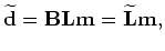
We re-write the linear modeling operation in equation (1) in matrix-vector form as follows:
 |
(4) |
where  is the modeling operator and
  is the earth reflectivity.
The encoding (or blending) operation in equation (2) is then defined as:
is the earth reflectivity.
The encoding (or blending) operation in equation (2) is then defined as:
 |
(5) |
where
 is the encoded data,
  is the encoding (or blending) operator, and
 is the combined modeling and encoding operator.
Given two surveys (baseline and monitor), acquired over an evolving earth model at times  and
and  respectively, we can write
 |
(6) |
where
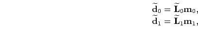 and
and
 are the baseline and monitor reflectivities, and
 and
and
 are the encoded seismic data sets.
Note that the modeling operators
are the encoded seismic data sets.
Note that the modeling operators
 and
and
 in equation (6) can define both different acquisition geometries and different relative shot-timings.
By applying the adjoint operators to the data sets, we obtain the migrated images:
 |
(7) |
where
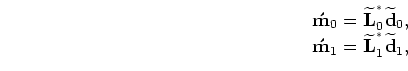 and
and
 are the migrated baseline and monitor images respectively, and the symbol
 denotes the conjugate transpose of the modeling operators.
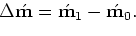
The raw time-lapse seismic image
denotes the conjugate transpose of the modeling operators.
The raw time-lapse seismic image
 is the difference between the migrated images:
 |
(8) |
Because of differences in relative shot-timings, cross-term artifacts (Romero et al., 2000; Tang and Biondi, 2009) will be different for each migrated data set.
Conventional equalization methods (Rickett and Lumley, 2001; Calvert, 2005) will be inadequate to remove these artifacts.
The quadratic cost functions for equation (6) are
 |
(9) |
which when minimized gives the inverted baseline
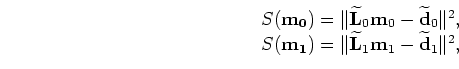 and monitor
 images:
 |
(10) |
This is the so-called data-space least-squares migration/inversion method.
Subsections
|
|
|
|
| Joint inversion of simultaneous source time-lapse seismic data sets | |
|
Next: Joint-inversion
Up: Ayeni et al.: Inversion
Previous: Linear phase-encoded Born modeling
2009-09-25