Automatic velocity picking by simulated annealing

2-D velocity model example

We apply the simulated annealing algorithm to the ELF7D data set. This dataset is complicated not only because of the salt dome, but also the complicated geological structure caused by the rising of the salt.

To optimize the velocity model, we use grid samplings of 63 $\times$ 266 m, and the number of grid points is 832. We start from a residual migration semblance cube. The residual migration parameter $\rho$ ranges from 0.925 to 1.0745. The aim of the algorithm is to produce a smooth and accurate velocity model in accordance with the semblance cube. We initialize the system with the $\rho$ values corresponding to semblance peaks, and randomly perturb the system through changing the $\rho$ value to any possible $\rho$ value defined by the residual migration. To create a smooth velocity model, we choose a much larger weight for smoothness than for semblance.

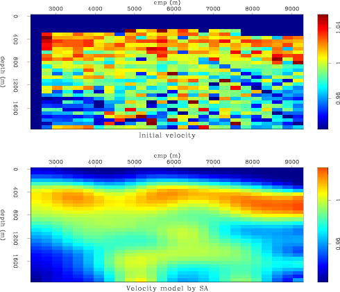
The result of the simulated annealing algorithm is shown in Figure 1. The model generated by 3200 iterations is much smoother than the initial model, but its main structure is still present in the final velocity model.

velocity-semb
Figure 1. Initial velocity model (top). Velocity model after 3200 iterations (bottom). The SA velocity is much smoother and still has the structure of the initial velocity model. [ER]

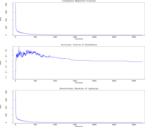
The top panel of Figure 2 shows the composite cost function while cooling. The cost function fluctuates up and down when the temperature is high, but the general trend is always decreasing. When the temperature is lower, the cost function goes down more steadily. As seen in the plot, the uphill perturbations are accepted less and less frequently by the Metropolis algorithm along the cooling path. Generally, the cost decreases much faster during the first iterations. As the annealing proceeds, the cost becomes more stable, until complete stability is reached at crystallization. The bottom two plots in Figure 2 show the cost curve of semblance and smoothness, respectively. Started from the minimum solution for semblance, simulated annealing maintains the increase of semblance within a factor of 2 while significantly enhancing the smoothness.

costpart
Figure 2. The plot on the top is the composite cost function; the plot in the middle is the cost of semblance; the plot at the bottom is the cost of smoothness. SA succeeds in controlling the increase of semblance when significantly enhancing smoothness. [ER]

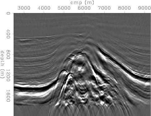
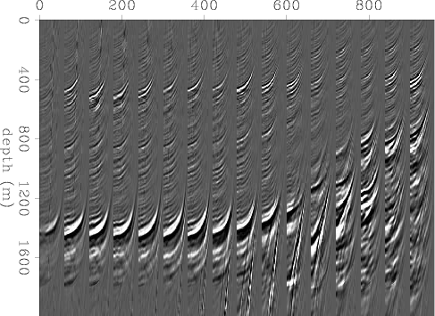
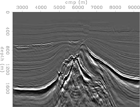
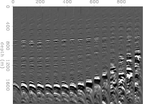
Figure 3 and Figure 5 show the migration images before and after SA velocity analysis, respectively. Figure 4 and Figure 6 show the corresponding angle domain common image gathers (ADCIGs). It can be seen that the corners of the geological structure are focused and the boundaries of the salt body are connected after the velocity update.

stack0
Figure 3. Migration image before performing SA velocity analysis. [ER]

cigplane0
Figure 4. Corresponding angle domain common image gathers of figure 3. [ER]

stack1
Figure 5. The residual migration image using the SA velocity model. Structures are well focused and the salt boundaries are connected. [ER]

cigplane1
Figure 6. Angle domain common image gathers according to SA velocity. They are not flat in the complex area. The smiling events above water bottom can be corrected by further contrails. [ER]

Automatic velocity picking by simulated annealing