|
|
|
|
Visualization and data reordering using EcoRAM |
Using this template, the transpose algorithm can be written in a push (loop
over input) or pull (loop over output) manner. For EcoRAM , and in many other
cases (such as wanting to pipe the output), the pull method is more efficient.
The basic transpose algorithm using the five dimensional template then
takes the following form.
![]()
This simple algorithm assumes that you can hold both the input and
output matrices in RAM. A problem with this simple approach is the
very poor use of input cache lines for small 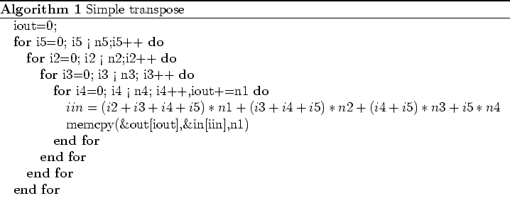 .
.
If we can hold ![]() is memory we can get acceptable performance
with either algorithm 4 or slight modification
that processes each
is memory we can get acceptable performance
with either algorithm 4 or slight modification
that processes each ![]() block in turn. We could still use the
basic template for large problems by mmapping the input and output file but
the cache miss problem would be further exacerbated. A better alternative
is to introduce two temporary buffers, tin and tout. These buffers
are of size
block in turn. We could still use the
basic template for large problems by mmapping the input and output file but
the cache miss problem would be further exacerbated. A better alternative
is to introduce two temporary buffers, tin and tout. These buffers
are of size ![]() , where
, where ![]() is chosen so that the combined
size of tin and tout does not exceed DRAM
is chosen so that the combined
size of tin and tout does not exceed DRAM![]() . The buffered algorithm
then takes the following form.
. The buffered algorithm
then takes the following form.
![]()
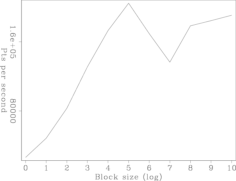
The larger ![]() , the better the performance. Figure 1 shows that even
a RAM-based system benefits from the buffered approach. Note how we can
gain a performance advantage of greater than six with larger
, the better the performance. Figure 1 shows that even
a RAM-based system benefits from the buffered approach. Note how we can
gain a performance advantage of greater than six with larger 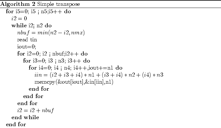 sizes.
|
ram
Figure 1. The number of elements per second vs |
|
|---|---|
|
|
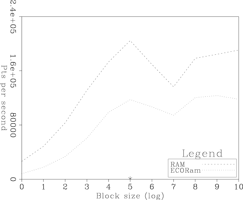
Figure 2 compares the performance of EcoRAM versus RAM. Note the
similarity of the two curves. The `*' in the figure shows the comparable
disk approach. The disk approach is ![]() th speed of the slowest
EcoRAM result and
th speed of the slowest
EcoRAM result and ![]() th the optimal buffer choice.
th the optimal buffer choice.
|
disk
Figure 2. The number of elements per second vs. |
|
|---|---|
|
|
As a final test, we transposed a float dataset of size
![]() switching
axes 1,2 with axis 5. Using the buffered approach of
algorithm 5, a conventional disk took 1293 minutes (using
an intermediate buffer size of 1 GB) while the same
dataset took 22 minutes using EcoRAM , a
switching
axes 1,2 with axis 5. Using the buffered approach of
algorithm 5, a conventional disk took 1293 minutes (using
an intermediate buffer size of 1 GB) while the same
dataset took 22 minutes using EcoRAM , a ![]() performance improvement.
performance improvement.
|
|
|
|
Visualization and data reordering using EcoRAM |