|
 |
 |
 | Modeling, migration, and inversion in the generalized source and receiver domain |  |
![[pdf]](icons/pdf.png) |
Next: encoded receivers
Up: Modeling, migration, and inversion
Previous: Born modeling and inversion
Let us define the encoding transform along the  coordinate of the surface data as follows:
 |
|
|
(A-8) |
where
 is the source phase-encoding function.
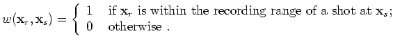
Equation 8 integrates along the horizontal dashed lines shown in Figure 1 for each receiver location
is the source phase-encoding function.
Equation 8 integrates along the horizontal dashed lines shown in Figure 1 for each receiver location  and
transforms the surface data from
and
transforms the surface data from
 domain into the
 domain.
For the plane-wave phase encoding, the encoding function is:
domain.
For the plane-wave phase encoding, the encoding function is:
 |
|
|
(A-9) |
where  is defined to be the ray parameter of the source plane waves. For random phase encoding, the encoding function is
 |
|
|
(A-10) |
where
 is a random sequence in and
  , and
defines the index of different realizations of the random sequence.
, and
defines the index of different realizations of the random sequence.
Substituting Equation 1 into 8, rearranging the order of summation, we get the forward modeling equation in the encoded source domain:
where the encoded source Green's function
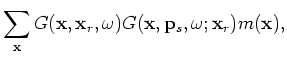 is defined as follows:
 |
|
|
(A-12) |
Note that
depends on because of the acquisition mask
 inside the summation.
It should only integrate the grey segment for each horizontal dashed line shown in Figure 1.
inside the summation.
It should only integrate the grey segment for each horizontal dashed line shown in Figure 1.
As derived in Appendix A, the objective function in the encoded source domain can be written as follows:
 |
|
|
(A-13) |
where 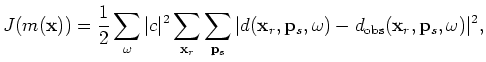 for plane-wave phase encoding, and
  for random phase encoding.
The gradient of the objective function in Equation 13 gives the following migration formula in the encoded source domain:
 |
|
|
(A-14) |
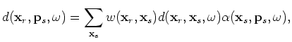
where the residual
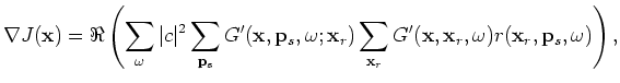 is defined as follows:
 |
(A-15) |
It is easy to see that Equation 14 defines the phase-encoding migration (Romero et al., 2000; Liu et al., 2006).
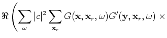
By taking the second-order derivatives of the objective function defined in Equation 13 with respect to the model paramters,
we obtain the Hessian in the encoded source domain:
|
|
|
|
| Modeling, migration, and inversion in the generalized source and receiver domain | |
|
Next: encoded receivers
Up: Modeling, migration, and inversion
Previous: Born modeling and inversion
2009-04-13