 |
 |
 |
 | Image-space wave-equation tomography in the generalized source domain |  |
![[pdf]](icons/pdf.png) |
Next: About this document ...
Up: Image-space wave-equation tomography in
Previous: APPENDIX B
This appendix demonstrates a matrix representation of the adjoint tomographic operator
 .
Since the slowness perturbation
.
Since the slowness perturbation
 is linearly related to the perturbed wavefields,
 and
and
 ,
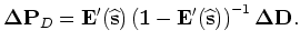
to obtain the back-projected slowness perturbation, we first must get the back-projected perturbed wavefields from the perturbed image
,
to obtain the back-projected slowness perturbation, we first must get the back-projected perturbed wavefields from the perturbed image
 .
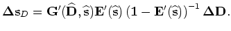
From Equation B-15, the back-projected perturbed source and receiver wavefields are obtained as follows:
.
From Equation B-15, the back-projected perturbed source and receiver wavefields are obtained as follows:
 |
|
|
(C-1) |
and
 |
|
|
(C-2) |
Then the adjoint equations of Equations B-10 and B-14 are
used to get the back-projected slowness perturbation
.
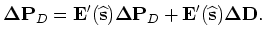
Let us first look at the adjoint equation of Equation B-10, which can be written as follows:
 |
|
|
(C-3) |
We can define a temporary wavefield
 that satisfies the following equation:
 |
|
|
(C-4) |
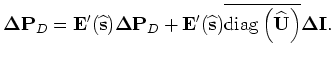
After some simple algebra, the above equation can be rewritten as follows:
 |
|
|
(C-5) |
Substituting Equation C-1 into equation C-5 yields
 |
|
|
(C-6) |
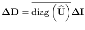
Therefore,
can be obtained by recursive upward continuation,
where
 serves as the initial condition.
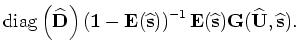
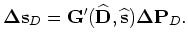
The back-projected slowness perturbation from the perturbed source wavefield is then obtained by applying the adjoint of the scattering
operator
serves as the initial condition.
The back-projected slowness perturbation from the perturbed source wavefield is then obtained by applying the adjoint of the scattering
operator
 to the wavefield
as follows:
to the wavefield
as follows:
 |
|
|
(C-7) |
Similarly, the adjoint equation of Equation B-14 reads as follows:
 |
|
|
(C-8) |
We can also define a temporary wavefield
 that satisfies the following equation:
 |
|
|
(C-9) |
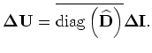
After rewriting it, we get the following recursive form:
The back-projected slowness perturbation from the perturbed receiver wavefield is then obtained by applying the adjoint of
the scattering operator
 to the wavefield
as follows:
to the wavefield
as follows:
 |
|
|
(C-11) |
The total back-projected slowness perturbation is obtained by adding
 and
and
 together:
 |
|
|
(C-12) |
|
|
|
|
| Image-space wave-equation tomography in the generalized source domain | |
|
Next: About this document ...
Up: Image-space wave-equation tomography in
Previous: APPENDIX B
2009-04-13