Image-space wave-equation tomography in the generalized source domain

APPENDIX B

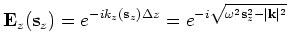
This appendix demonstrates a matrix representation of the forward tomographic operator ${\bf T}$. Let us start with the source wavefield, where the source wavefield ${\bf D}_z$ at depth $z$ is downward continued to depth $z+\Delta z$ by the one-way extrapolator ${\bf E}_z({\bf s}_z)$ as follows:

$${\bf D}_{z+\Delta z} = {\bf E}_z({\bf s}_z){\bf D}_z,$$ (B-1)

where the one-way extrapolator is defined as follows:

$${\bf E}_{z}({\bf s}_z) = e^{-ik_z({\bf s}_z)\Delta z} = e^{-i\sqrt{\omega^2{\bf s}_z^2-\vert{\bf k}\vert^2}}$$ (B-2)

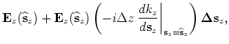
The perturbed source wavefield at some depth level can be derived from the background wavefield by a simple application of the chain rule to equation B-1:

$${\bf\Delta D}_{z+\Delta z} = {\bf E}_z({\widehat{\bf s}}_z){\bf\Delta D}_z + {\bf\Delta E}_z({\widehat{\bf s}}_z)\widehat{{\bf D}}_z,$$ (B-3)

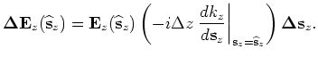
where $\widehat{{\bf D}}_z$ is the background source wavefield and ${\bf\Delta E}_z$ represents the perturbed extrapolator, which can be obtained by a formal linearization with respect to slowness of the extrapolator defined in Equation B-2:

$${\bf E}_z({\bf s}_z) = e^{-ik_z({\bf s}_z)\Delta z} \approx e^{-i\Delta z {\widehat k_z}} + e^{-i\Delta z {\widehat k_z}}\lef... ...\bf s}_z} \right\vert _{{\bf s}_z={\widehat {\bf s}}_z} \right) {\bf\Delta s}_z$$

$$= {\bf E}_z(\widehat{{\bf s}}_z) + {\bf E}_z(\widehat{{\bf s}}_z) \... ...\bf s}_z} \right\vert _{{\bf s}_z={\widehat {\bf s}}_z}\right) {\bf\Delta s}_z,$$ (B-4)

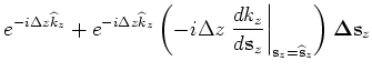
where ${\widehat k}_z=k_z({\widehat {\bf s}}_z)$ and $\widehat{{\bf s}}_z$ is the background slowness at depth $z$. From Equation B-4, the perturbed extrapolator reads as follows:

$${\bf\Delta E}_z({\widehat {\bf s}}_z) = {\bf E}_z(\widehat{{\bf s... ...\bf s}_z} \right\vert _{{\bf s}_z={\widehat {\bf s}}_z}\right) {\bf\Delta s}_z.$$ (B-5)

Substituting Equation B-5 into B-3 yields

$${\bf\Delta D}_{z+\Delta z} = {\bf E}_z({\widehat{\bf s}}_z){\bf\D... ...t _{{\bf s}_z={\widehat {\bf s}}_z}\right) \widehat{{\bf D}}_z {\bf\Delta s}_z.$$ (B-6)

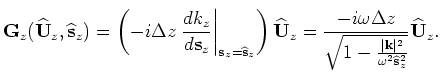
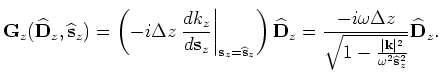
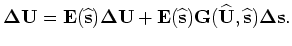
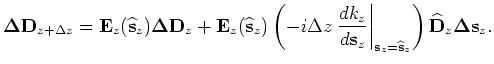
Let us define a scattering operator ${\bf G}_z$ that interacts with the background wavefield as follows:

$${\bf G}_z(\widehat{{\bf D}}_z,{\widehat {\bf s}}_z) = \left( - i\... ...c{\vert{\bf k}\vert^2}{\omega ^2 {\widehat {\bf s}}_z^2}}} \widehat{{\bf D}}_z.$$ (B-7)

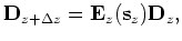
Then the perturbed source wavefield for depth $z+\Delta z$ can be rewritten as follows:

$${\bf\Delta D}_{z+\Delta z} = {\bf E}_z({\widehat {\bf s}}_z){\bf\... ...bf s}}_z) {\bf G}_z({\widehat {\bf D}}_z,{\widehat {\bf s}}_z) {\bf\Delta s}_z.$$ (B-8)

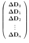
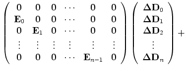
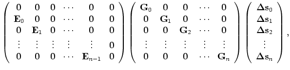
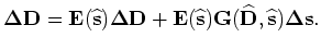
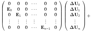
We can further write out the recursive Equation B-8 for all depths in the following matrix form:

$$\left( \begin{array}{c} {\bf\Delta D}_0 \\ {\bf\Delta D}_1 \\ {\bf\Delta D}_2 \\ {\vdots}\\ {\bf\Delta D}_n \end{array} \right) = \left( \begin{array}{cccccc} {\bf0} & {\bf0} & {\bf0} & {\cdots} ... ... D}_1 \\ {\bf\Delta D}_2 \\ {\vdots}\\ {\bf\Delta D}_n \end{array} \right) +$$

$$\left( \begin{array}{cccccc} {\bf0} & {\bf0} & {\bf0} & {\cdots} ... ...a s}_1 \\ {\bf\Delta s}_2 \\ {\vdots}\\ {\bf\Delta s}_n \end{array} \right),$$

or in a more compact notation,

$${\bf\Delta D} = {\bf E}({\widehat {\bf s}}){\bf\Delta D} + {\bf E}({\widehat {\bf s}}){\bf G}({\widehat {\bf D}},{\widehat {\bf s}}){\bf\Delta s}.$$ (B-9)

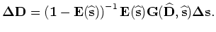
The solution of Equation B-9 can be formally written as follows:

$${\bf\Delta D} = \left( {\bf 1} - {\bf E}({\widehat {\bf s}}) \rig... ...{\widehat {\bf s}}){\bf G}({\widehat {\bf D}},{\widehat {\bf s}}){\bf\Delta s}.$$ (B-10)

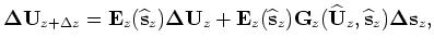
Similarly, the perturbed receiver wavefield satisfies the following recursive relation:

$${\bf\Delta U}_{z+\Delta z} = {\bf E}_z({\widehat {\bf s}}_z){\bf\... ... s}}_z) {{\bf G}_z({\widehat {\bf U}}_z,{\widehat {\bf s}}_z)} {\bf\Delta s}_z,$$ (B-11)

where ${\bf G}_z({\widehat {\bf U}}_z,{\widehat {\bf s}}_z)$ is the scattering operator, which interacts with the background receiver wavefield as follows:

$${\bf G}_z({\widehat {\bf U}}_z,{\widehat {\bf s}}_z) = \left( - i... ...{\vert{\bf k}\vert^2}{\omega ^2 {\widehat {\bf s}}_z^2}}} {\widehat {\bf U}}_z.$$ (B-12)

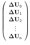
We can also write out the recursive Equation B-12 for all depth levels in the following matrix form:

$$\left( \begin{array}{c} {\bf\Delta U}_0 \\ {\bf\Delta U}_1 \\ {\bf\Delta U}_2 \\ {\vdots}\\ {\bf\Delta U}_n \end{array} \right) = \left( \begin{array}{cccccc} {\bf0} & {\bf0} & {\bf0} & {\cdots} ... ... U}_1 \\ {\bf\Delta U}_2 \\ {\vdots}\\ {\bf\Delta U}_n \end{array} \right) +$$

$$\left( \begin{array}{cccccc} {\bf0} & {\bf0} & {\bf0} & {\cdots} ... ...a s}_1 \\ {\bf\Delta s}_2 \\ {\vdots}\\ {\bf\Delta s}_n \end{array} \right),$$

or in a more compact notation,

$${\bf\Delta U} = {\bf E}({\widehat {\bf s}}){\bf\Delta U} + {\bf E}({\widehat {\bf s}}){\bf G}({\widehat {\bf U}},{\widehat {\bf s}}){\bf\Delta s}.$$ (B-13)

The solution of Equation B-13 can be formally written as follows:

$${\bf\Delta U} = \left( {\bf 1} - {\bf E}({\widehat {\bf s}}) \rig... ...\widehat {\bf s}}) {\bf G}({\widehat {\bf U}},{\widehat {\bf s}}){\bf\Delta s}.$$ (B-14)

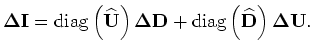
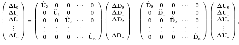
With the background wavefields and the perturbed wavefields, the perturbed image can be obtained as follows:

$$\left( \begin{array}{c} {\bf\Delta I}_0 \\ {\bf\Delta I}_1 \\ {... ...}_1}\\ {{\bf\Delta U}_2}\\ {\vdots}\\ {{\bf\Delta U}_n} \end{array} \right),$$

or in a more compact notation,

$${\bf\Delta I} = {\rm diag}\left({\widehat {\bf U}}\right){\bf\Delta D} + {\rm diag}\left( {\widehat{\bf D}}\right){\bf\Delta U}.$$ (B-15)

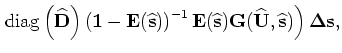
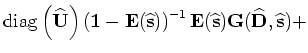
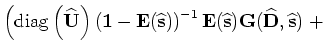
Substituting Equations B-10 and B-14 into Equation B-15 yields

$${\bf\Delta I} = \left( {\rm diag}\left( {\widehat {\bf U}}\right) \left( {\bf 1} ... ... E}({\widehat {\bf s}}){\bf G}({\widehat {\bf D}},{\widehat {\bf s}}) \right. +$$

$$\left. {\rm diag}\left({\widehat {\bf D}} \right) \left( {\bf 1} ... ...t {\bf s}}){\bf G}({\widehat {\bf U}},{\widehat {\bf s}}) \right){\bf\Delta s},$$ (B-16)

from which we can read the forward tomographic operator ${\bf T}$ as follows:

$${\bf T} = {\rm diag}\left( {\widehat {\bf U}}\right) \left( {\bf 1} - {\bf ... ...-1} {\bf E}({\widehat {\bf s}}){\bf G}({\widehat {\bf D}},{\widehat {\bf s}}) +$$

$${\rm diag}\left({\widehat {\bf D}} \right) \left( {\bf 1} - {\bf ... ...{-1} {\bf E}({\widehat {\bf s}}){\bf G}({\widehat {\bf U}},{\widehat {\bf s}}).$$ (B-17)

Image-space wave-equation tomography in the generalized source domain