3D pyramid interpolation

Patch from the qdome data set

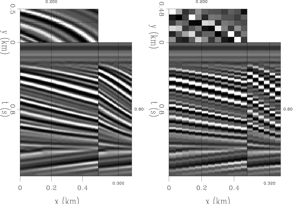
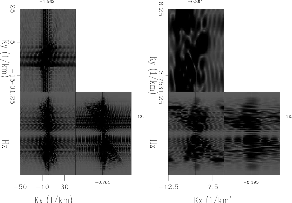
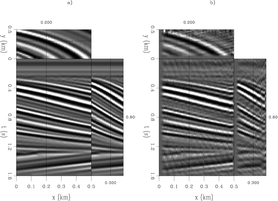
In this example, I windowed out one fourth of the qdome data set, in which the reflectors are almost stationary (Figure 6 a). I then sub-sampled the data cube by a factor of four along both the $x$ and $y$ axes (Figure 6 b). This caused aliasing of some reflectors, especially in the cross line direction, as the $f$-$\bf k$ spectrum of Figure 7 shows. Since this data set is more complicated then the previous one, and not all the reflectors are ideally stationary, in the pyramid domain, I use ten as the sampling factor along both $x$ and $y$ directions to make sure low frequency data are well represented. Then with the initial guess of the PEF also being 2D Laplacian operator, the above algorithms converged to a satisfactory result for most of the reflectors (Figure 8b ). Notice that for reflectors with small amplitude, the interpolation works not so well, and tuning the PEF size may help solving this problem. By looking at the the depth slice in Figure 8b , zeros can be observed for data at small $x$ and $y$ values, this is due to insufficient number of data points for PEF estimation at these locations. On the other hand, the other two edges have much stronger amplitude artifacts, which requires further investigation.

qd
Figure 6. a) Original patch of qdome data, where all the reflectors are almost stationary. b) Sub-sampling by a factor of four along both the $x$ and $y$ axes. [ER]

wkqd
Figure 7. a) The $f$-$k$ spectrum of the original data. b) The $f$-$k$ spectrum of the sub-sampled data. [ER]

qdi
Figure 8. a) Original patch of qdome data. b) Interpolated data. [CR]

3D pyramid interpolation