Angle-domain common-image gathers in generalized coordinates

Test 1: Elliptic Isochrons

The first test demonstrates the impulse response of the ADCIG imaging operator. I do this by imaging the elliptic isochronal responses of two offset point sources in a constant velocity medium (see Figure 4). The source wavefield impulse is at time $t=0$ s and at $x=-1.12$ km, while the receiver wavefield impulses are at $t=2.0$, 2.5, 3.0, and 3.5 s and $x=1.12$ km for a total source-receiver offset of $2h=2.24$ km. Correlating these two wavefield volumes leads to four elliptic isochrons specified by

$$x_1 (t,h) = \frac{vt}{4} \left( {\rm cos} \theta_1 + {\rm cos} \theta_2 \right)$$ (23)

$$x_3 (t,h) = \frac{vt}{4} \left(1 - \frac{h^2}{v^2t^2} \right) \left( {\rm sin} \theta_1 + {\rm sin} \theta_2 \right),$$ (24)

where, given the source take-off angle $\theta_1$, the receiver take-off angle $\theta_2$ is obtained by

$$\theta_2 = {\rm cos}^{-1} \left( \frac{vt}{2h} \left[ \frac{1}{\f... ...v^2t^2}} - \frac{1}{1-\frac{2h {\rm cos} \theta_1}{vt}} } -1 \right] \right).$$ (25)

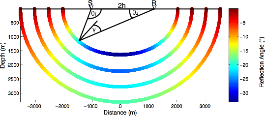
The reflection opening angle, given by $\gamma = 90 - \frac{(\theta_1 +\theta_2)}{2}$, is shown color-coded on the scatterplot in Figure 4.

Theory
Figure 4. Theoretical results for an elliptic isochron for four travel times in a constant velocity medium. The elliptic surfaces are color-coded according to reflection opening angle.

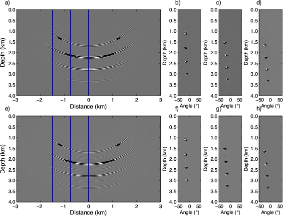
Figure 5 shows the ADCIG volumes calculated in both (a single) elliptic and Cartesian coordinate system. To generate this image, I first calculated an elliptic coordinate (EC) volume $I(\xi_1,\xi_3,h_{\xi_1})$ by correlating the source and receiver wavefields at 64 subsurface shifts in $h_{\xi _1}$ at each point in every extrapolation step. I then input the ODCIG volume to a Fourier-based offset-to-angle transformation operator to generate the EC ADCIG volume, $I(\xi_1,\xi_3,\gamma)$, which I interpolated to Cartesian coordinates to generate the desired image volume, $I(x_1,x_3,\gamma)$. For the ADCIG transformation, I choose to limit the maximum opening angle to $\gamma =\pm 60^\circ$. Thus, the 64 image shifts lead to ADCIGs with an angular range between $-60^\circ < \gamma < 60^\circ$ with a sampling increment of $\Delta \gamma = 1.875^\circ$.

Panel 5a presents the elliptic coordinate image extracted at $\gamma=-24^\circ$ from the ADCIG volume $I(x_1,x_3,\gamma)$. The ADCIG volumes consist of elliptically shaped reflectors (panels 5a) that are ideally localized in the angle domain (panels 5b-c and f-h). The analytical ADCIG locations are represented by black dots. The analytically and numerically generated results are well matched. Figure 5a also shows three vertical lines indicating the locations from left to right of the three ADCIGs in panels 5b-d. Again, the analytic and numerical ADCIGs are well matched, though less so at shallower depths due to the increased smearing about the image point in the $I(\xi_1,\xi_3,h_{\xi_1})$ domain (, ).

The Cartesian coordinate (CC) ADCIGs are presented in panels 5e-h. Panel 5e shows the Cartesian image again extracted at $\gamma=-24^\circ$ in the angle domain. Panels 5f-h present three ADCIGs at the same locations as in panels 5b-d. The Cartesian image volumes are well-matched to the elliptic coordinate examples, and good agreement between the theoretical results and the wavefield volume is observed in both images. Energy is focused in the neighborhood of the correct locations. The angle gathers are not always centered relative to the true location, though, which is more noticeable at shallower depths where the Cartesian and elliptic ADCIG volumes both overestimate the reflection opening angle.

EllipticTest
Figure 5. Elliptic reflector comparison tests between analytically (black bullets) and numerically generated ADCIG volumes. Panels a-d are computed in elliptic coordinates (EC), while panels e-h are in Cartesian coordinates (CC). a) EC image extracted at the -24$^\circ$ reflection angle. b) EC angle gather at -1.5 km. c) EC gather at 0.75 km. d) EC gather at 0.0 km. e) CC image extracted at the -24$^\circ$ reflection angle. f) CC angle gather at -1.5 km. g) CC gather at 0.75 km. h) CC gather at 0.0 km.

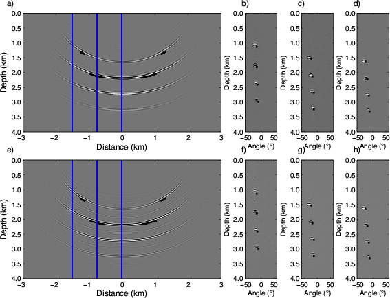
Figure 6 presents the results of a test similar to that shown in Figure 5, but with the velocity model rescaled by 0.98. Again, the black dots show the location of the true image point (assuming a true velocity model). Note that the image points in each ADCIG remain well-focused, but shift nearer to the surface and to wider angles. Thus, imaging with an overly slow velocity model will generate, as expected, reflectors that exhibit upward curvature at wider angles.

WrongEllipticTest
Figure 6. Elliptic reflector comparison tests between analytically (black bullets) and numerically generated ADCIG volumes using a velocity scaled by factor 0.98. Panels a-d are computed in elliptic coordinates (EC), while panels e-h are in Cartesian coordinates (CC). a) EC image extracted at the -24$^\circ$ reflection angle. b) EC angle gather at -1.5 km. c) EC gather at 0.75 km. d) EC gather at 0.0 km. e) CC image extracted at the -24$^\circ$ reflection angle. f) CC angle gather at -1.5 km. g) CC gather at 0.75 km. h) CC gather at 0.0 km.

Angle-domain common-image gathers in generalized coordinates