Ignoring density in waveform inversion

Application to models with and without density

To test effects of density on waveform inversion, we construct two earth models, one with reflectors simulated by velocity spikes and one with reflectors simulated by density spikes. We add a Gaussian anomaly to both velocity models to test whether our constant-density implementation of waveform inversion can recover long-wavelength velocity perturbations.

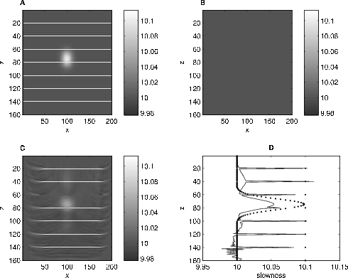
Figure 1 shows the slowness field (a) for the constant-density model. Ten horizontal stripes with +1% change in slowness act as reflectors that generate events in the data. Though the goal of waveform inversion is to invert long-wavelength velocity perturbations, the inversion also needs to recover high-frequency perturbations in order to match the data. We also add a +1% Gaussian anomaly to the model. We provide the inversion with a constant-slowness initial model (b) that matches the background velocity of the actual model. After 185 iterations, the inversion (c) recovers both the reflectors and the Gaussian anomaly. Vertical slices through the middle of the slowness model and inversion result (d) show that the inversion comes close to correctly estimating the magnitude of the slowness spikes, especially in the region unaffected by the anomaly. The inversion under-estimates the magnitude of the slowness anomaly, and it smears the anomaly vertically. These two effects tend to counteract each other since a slowness perturbation with a large spatial extent but small magnitude can introduce similar delays as a spatially small perturbation with a large magnitude.

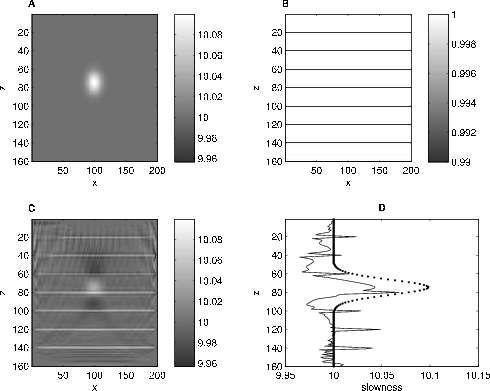
Figure 2 shows the slowness field (a) and the density field (b) for the variable-density model. In this example we introduce the same +1% Gaussian anomaly to the velocity model, but we simulate reflectors with density contrasts instead of slowness contrasts. Since slowness and density changes create reflections of opposite polarity, we add -1% spikes to the density model. After 300 iterations, the inversion introduces horizontal stripes into the velocity model to account for the density reflectors and partially recovers the Gaussian anomaly (c). Overall, the inversion result is noisier, and the norm of the data residual is larger than for the previous example. Vertical slices through the model and inversion result (d) show that the inversion introduces negative changes at the top and bottom of the anomaly, which is entirely positive. This example illustrates that data effects due to density can inhibit the ability of waveform inversion to recover velocity anomalies.

fig-vel
Figure 1. Numerical experiment for a constant-density earth: (a) slowness model use to compute the data; (b) starting slowness model; (c) inversion result after 185 iterations; and (d) slices through the model (dotted line) and inversion result (solid line).

fig-den
Figure 2. Numerical experiment for a variable-density earth. Data is modeled for a constant-background slowness field (a) containing a Gaussian anomaly but no reflectors. The reflectors are instead embedded in the density field (b). After 300 iterations, the inversion (c) attempts to fit the reflection with velocity spikes but still manages to recover some of the anomaly. (d) Slices through the model (dotted line) and inversion result (solid line) show that the anomaly is recovered less effectively than in the previous example.

Ignoring density in waveform inversion