Plane-wave migration in tilted coordinates

Plane-wave migration in tilted coordinates

We introduced the concepts of plane-wave migration and migration in tilted coordinates in previous sections. In this section, we discuss the combination of these two and provide a powerful method for migrating steeply dipping and overturned events. We first discuss why point-source migration in tilted coordinates would not be effective. Then we describe how to design tilted coordinates for each plane-wave source. Finally, we discuss how reciprocity improves plane-wave migration in tilted coordinates.

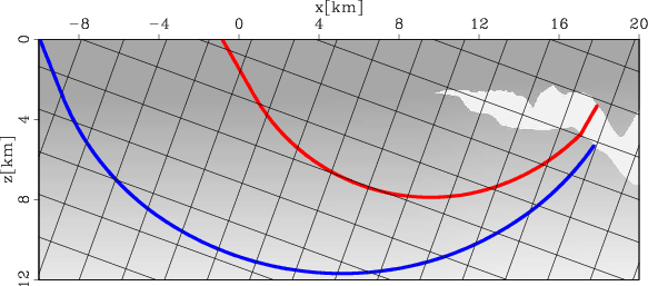
zigvelwithraytilt Figure 4. The velocity model and overturned waves in a tilted coordinate system. The overturned waves in vertical Cartesian coordinates do not overturn in the tilted coordinate system.

Waves from a point source propagate radially, and waves start from one spatial location and travel along all directions. Therefore, it is impossible for a tilted coordinate system to cover all the propagation directions of a point source. Figure 5a illustrates the waves from a point source in tilted coordinates. In Figure 5a the coordinates $(x,z)$ are rotated counter-clockwise, where the high-angle energy can be well modeled on the right side, but the left-side energy (represented by dash-lines) cannot be modeled accurately, even for small-angle energy in vertical Cartesian coordinates. However, the propagation direction of a plane-wave source at different spatial locations is usually similar (Figure 5b). In plane-wave migration, we decompose the wavefield into plane-wave source gathers by slant-stacking, and each plane-wave source gather is characterized by a ray-parameter $p_x$. Given the velocity at the surface $v_{z_0}$, the propagation direction of the plane-wave source is defined by the vector $(q_x,q_z)$, where $q_x=p_xv_{z_0}$ and $q_z=\sqrt{1-q_x^2}$. Therefore, the ray parameter $p_x$ defines the propagation direction of the plane-wave source at the surface. The take-off angle $\alpha$ of the plane-wave source can be calculated as follows:

$$\alpha=\arccos (q_x).$$ (15)

If we assume the velocity to be invariant at the surface, the propagation direction of the plane-wave source defined in equation 7 at the surface is the same for all spatial points. This is true for a marine dataset, and nearly true for a land dataset, if the velocity does not vary strongly at the surface. Therefore, a tilted coordinate system can cover most of the propagation directions of a plane-wave source from different spatial points, although the propagation direction of the plane-wave may change due to velocity heterogeneities.

pointplane Figure 5. Point source (a) and plane-wave sources (b) in tilted coordinates. Waves from a point source propagate radially, and the waves represented by the dash line rays in panel (a) can not be caught when we rotate the coordinates counter-clockwise. In contrast, the propagation directions of the plane-wave source are similar in different spatial points, so most of them can be extrapolated accurately in a tilted coordinate system.

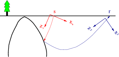
Given a plane-wave source with a take-off angle of $\alpha$, we use tilted coordinates $(x^\prime ,z^\prime )$, with a tilting angle $\theta$ close to its take-off angle $\alpha$. Usually, velocity increases with depth and the propagation direction of waves becomes increasingly horizontal, so in practice the tilting angle $\theta$ is a little larger than the take-off angle. Figure 6 shows three typical plane-wave sources and their tilted coordinate systems. Plane-wave sources with a small take-off angle mainly illuminate reflectors that are almost flat, so we extrapolate wavefields vertically. In contrast, plane-wave sources with a large take-off angle mainly illuminate steeply dipping reflectors, so we use a tilted coordinate system with a large tilting angle. Usually, these wavefields are difficult to extrapolate accurately by downward continuation migration, but in tilted coordinates their propagation direction is close to the extrapolation direction, so they can be imaged correctly. Waves overturning in vertical Cartesian coordinates do not overturn in a well-chosen tilted coordinate system. Therefore, in plane-wave migration in tilted coordinates, each plane-wave source has its own tilted coordinate system in which the extrapolation direction is close to the propagation direction, and steep reflectors and overturned waves can be imaged correctly.

planetilt Figure 6. Plane-wave sources and their tilted coordinates. The tilting direction for the coordinates corresponding to the plane-wave source depends on its take-off angle. There are three typical plane-wave sources, and they have 0, negative and positive ray parameters, respectively. For $p=0$, we use conventional Cartesian coordinates. For $p>0$, we rotate coordinates counter-clockwise and for $p<0$, we rotate coordinates clockwise.

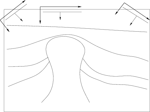
reciprocity
Figure 7. Reciprocity improves plane-wave migration in tilted coordinates. The source location is at $s$, and the receiver location is at $r$. For this event, the source ray does not overturn, but the receiver ray does. If we run plane-wave migration in tilted coordinates on the original one-sided offset data, we will use the coordinates $(x_s,z_s)$, whose direction is determined by the source ray direction at the surface. In this coordinate system, the source waves can be handled but the overturned receiver wave cannot. If we run the same migration on the other side offset data generated by reciprocity, we will use the coordinates $(x_r,z_r)$ for wavefield extrapolation, whose direction is determined by the receiver ray direction at the surface. In this coordinate system, both the source and receiver waves can be handled.

Usually, in streamer acquisition we only record one-sided offset data at the surface. But we can obtain the data for the other side by reciprocity. Merging the original data and the data obtained by reciprocity, we obtain a dataset that would be recorded if we would have had a split-spread recording geometry. In plane-wave migration for a dataset with a split-spread geometry, the aperture of each plane-wave source is almost the same as one-sided offset dataset, and thus the computation cost is also almost the same. But a split-spread recording geometry improves the plane-wave gathers and the signal-to-noise ratio of the image (Liu et al., 2006).

Reciprocity yields other benefits for plane-wave migration in tilted coordinates. Figure 7 illustrates how reciprocity helps to image steep salt flanks when the source ray does not overturn but the receiver ray does. In Figure 7, the source location is $s$ and receiver location is $r$. For the original data, we run plane-wave migration for this event using the coordinates $(x_s,z_s)$, whose tilting angle is determined by the source ray direction at the surface. The source plane wave starts at the surface almost vertically, and the tilting angle of its corresponding coordinates $(x_s,z_s)$ is small. As a consequence, the overturned receiver wave cannot be accurately modeled, and the event cannot be correctly imaged. Reciprocity exchanges the source and receiver locations. For the data obtained by reciprocity, we run plane-wave migration for this event using the coordinates $(x_r,z_r)$, whose direction is determined by the receiver ray direction at the surface. In the coordinates $(x_r,z_r)$, both source and receiver waves can be accurately modeled, and the overturned energy can be correctly imaged. When we run plane-wave migration in tilted coordinates for a split-spread dataset, we design the coordinates considering the direction of both the source and receiver waves at the surface.

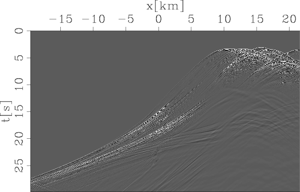
zigdata
Figure 8. The exploding reflector dataset from the revised Sigsbee 2A model. The overturned energy is recorded from $-20$ to $5$km at $t=10$ to $25$ s. The energy recorded earlier than $10$ s is muted before migration to verify the imaging of overturned waves.

zigimage
Figure 9. Migrated image of the overturned waves: migration in tilted coordinates (a) and reverse-time migration (b).

Plane-wave migration in tilted coordinates