 |
 |
 |
 | Plane-wave migration in tilted coordinates |  |
![[pdf]](icons/pdf.png) |
Next: Plane-wave migration in tilted
Up: Shan and Biondi: Plane-wave
Previous: Plane-wave source migration
The extrapolation direction plays a key role in one-way wave-equation wavefield extrapolation,
since the waves traveling along the extrapolation direction are modeled the most accurately.
However, the extrapolation direction has no physical meaning and it is only a direction artificially assigned in numerical algorithms.
In conventional downward continuation migration, we use vertical Cartesian coordinates and extrapolate wavefields vertically.
The extrapolation direction can be changed by rotating the coordinates.
It is well known that the acoustic equation (equation 1) is invariant to coordinate rotations as follows:
 |
(11) |
We call the new coordinate system
 a tilted Cartesian coordinate system (or tilted coordinate system) and
the angle
a tilted Cartesian coordinate system (or tilted coordinate system) and
the angle 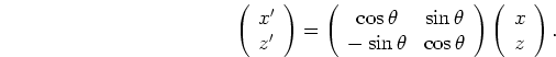 the tilting angle for the coordinate system.
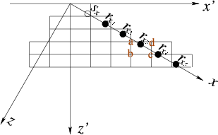
tiltcoordinate1
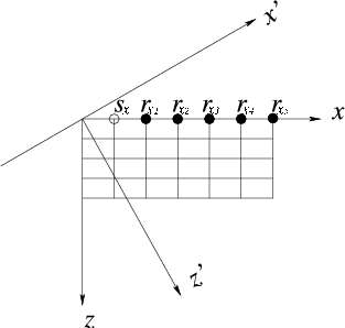
Figure 1. Coordinate system rotation:
 are conventional vertical Cartesian coordinates,
are tilted coordinates, are conventional vertical Cartesian coordinates,
are tilted coordinates,  represents the source location,
and represents the source location,
and
 represent receiver locations. The source and receivers are on regular grids in vertical Cartesian coordinates. represent receiver locations. The source and receivers are on regular grids in vertical Cartesian coordinates.
|
|
![[png]](icons/viewmag.png)
|
|---|
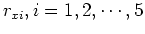
As in the vertical Cartesian coordinates, the up-going and down-going one-way wave equations can be obtained by splitting the acoustic wave equation
in the tilted coordinate system
:
 |
|
|
(12) |
 |
|
|
(13) |
The extrapolation direction of equations 12 and 13
parallels the 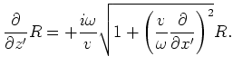 axis, which is from the vertical direction.
Figure 1 illustrates the coordinate transformation, where are vertical Cartesian coordinates and
are tilted coordinates, represents the source location and
axis, which is from the vertical direction.
Figure 1 illustrates the coordinate transformation, where are vertical Cartesian coordinates and
are tilted coordinates, represents the source location and
 represent the corresponding receiver locations.
The accuracy of the one-way wavefield extrapolators is still very important for wavefield extrapolation in tilted coordinates.
The more accurately we design the wavefield extrapolator, the less sensitive the migration is to the coordinates.
With an extrapolator that is not very accurate, such as the
represent the corresponding receiver locations.
The accuracy of the one-way wavefield extrapolators is still very important for wavefield extrapolation in tilted coordinates.
The more accurately we design the wavefield extrapolator, the less sensitive the migration is to the coordinates.
With an extrapolator that is not very accurate, such as the  equation,
waves well handled in one coordinate system are not handled in one that is slightly rotated.
In contrast, with an accurate extrapolator, waves can be handled in both tilted coordinate systems.
Since one-way wave equations in tilted coordinates are exactly the same as those in vertical
Cartesian coordinates, all the methods used to improve the accuracy in the conventional Cartesian coordinates still work in tilted coordinates.
equation,
waves well handled in one coordinate system are not handled in one that is slightly rotated.
In contrast, with an accurate extrapolator, waves can be handled in both tilted coordinate systems.
Since one-way wave equations in tilted coordinates are exactly the same as those in vertical
Cartesian coordinates, all the methods used to improve the accuracy in the conventional Cartesian coordinates still work in tilted coordinates.
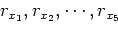
tiltcoordinate2
Figure 2. Source and receivers in grids of a tilted coordinate
system: are conventional vertical Cartesian coordinates,
are tilted coordinates, represents the source location, and
represent receiver locations.
Neither source nor receiver locations are on regular grids in the tilted coordinate system.
Their wavefield values must be interpolated onto regular grids around the slanted line in tilted coordinates. The wavefield on  is interpolated onto the grids a, b, c, and d. is interpolated onto the grids a, b, c, and d.
|
|
|
|
|---|
To extrapolate wavefields in a tilted coordinate system, it is necessary to interpolate
the surface dataset, velocity model and image between the coordinate systems and migrate the dataset on a slanted line in implementation.
In Figure 1, the source and receivers are on regular grids in conventional Cartesian coordinates. Figure 2 shows the source and receivers in
meshes in the tilted coordinates
. Source and receivers are on an inclined line defined by the equation
 |
(14) |
They are not on regular grids in tilted coordinates. To run wavefield extrapolation, the dataset received at the surface
has to be interpolated onto the regularized grids around the inclined line in the new coordinate system
.
For instance, the value of the wavefield at  has to be interpolated onto the grids a,b,c and d in Figure 2.
The velocity must also be interpolated onto the grids in the coordinates
.
In tilted coordinates, the survey is taken on a long, slanted line defined by equation 14.
We extrapolate the wavefield with the surface dataset on the slanted line injected at each depth step.
We begin the wavefield extrapolation at the point
has to be interpolated onto the grids a,b,c and d in Figure 2.
The velocity must also be interpolated onto the grids in the coordinates
.
In tilted coordinates, the survey is taken on a long, slanted line defined by equation 14.
We extrapolate the wavefield with the surface dataset on the slanted line injected at each depth step.
We begin the wavefield extrapolation at the point  . For the
  -th step extrapolation,
when the depth level
-th step extrapolation,
when the depth level
 intersects the slanted line,
we add the measured wavefield on the slanted line to the wavefield extrapolated from its previous depth level. After we inject the wavefields on the
slanted line, the wavefield extrapolation is the same as the conventional one.
intersects the slanted line,
we add the measured wavefield on the slanted line to the wavefield extrapolated from its previous depth level. After we inject the wavefields on the
slanted line, the wavefield extrapolation is the same as the conventional one.
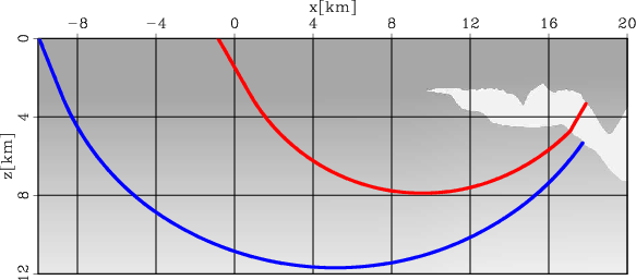
Figure 3 shows a velocity model revised from the Sigsbee 2A model (Sava, 2006). The sediment part of the model is
extended vertically and horizontally to receive the overturned waves from the overhanging salt flank at the surface.
The rays correspond to the overturned waves from the overhanging flanks on opposite sides of the salt. Figure 4 shows the model
and rays in a tilted coordinate system with a tilting angle of  . Figures 3 and
4 illustrate that the waves that overturn in vertical Cartesian coordinates do not overturn
in a tilted coordinate system with a well-chosen tilting direction.
. Figures 3 and
4 illustrate that the waves that overturn in vertical Cartesian coordinates do not overturn
in a tilted coordinate system with a well-chosen tilting direction.
zigvelwithraycart
Figure 3. A velocity model revised from Sigsbee 2A. The sediment parts of the model are extended to
allow the overturned waves from the overhanging salt flanks to be received at the surface.
The rays represent the overturned waves
from the overhanging salt flank.
|
|
|
|
|---|
|
|
|
|
| Plane-wave migration in tilted coordinates | |
|
Next: Plane-wave migration in tilted
Up: Shan and Biondi: Plane-wave
Previous: Plane-wave source migration
2007-09-18