Circuit Design

The mapping from the software code to a hardware circuit design is straightforward for most parts. Fig. 4 shows the general structure of the circuit design. Compared with the software Fortran code shown above, one big difference is the handling of the sine and cosine functions. In the software code, the trigonometric functions are calculated outside of the five-level loop, and stored as a look-up table. In the hardware design, to take advantage of the parallel calculation capability provided by the numerous logic units on the FPGA, the calculation of the sine/cosine functions are merged into the processing core of the inner loop. Three function evaluation units are included in this design, to produce values for the square root, cosine and sine functions separately. As mentioned in earlier, all three functions are evaluated using degree-one polynomial approximation with 386 to 512 uniform segments.

The other task in the hardware circuit design is to map the calculation into arithmetic operations of certain number representations. The previous table shows the value range of some typical variables in the `wei_wem' function. Some of the variables (in the part of square root and sine/cosine function evaluations) have a small range within [0, 1], while other values (especially `wfld' data) have a wider range from $10^{-14}$ to

. If we use floating-point or LNS number representations, their wide representation ranges are enough to handle these variables. However, if we use fixed-point number representations in the design, special handling is needed to achieve acceptable accuracy over wide ranges.

Table 1: Profiling results for the ranges of typical variables in function `wei_wem'. `wfld_real' and `wfld_img' refer to the real and imaginary parts of the `wfld' data. `Max' and `Min' refer to the maximum and minimum absolute values of variables.

Variable	step%x	ko	wfld_real	wfld_img
Max	0.377	0.147	3.918e6	3.752e6
Min	0	7.658e-3	4.168e-14	5.885e-14

The first issue to consider in fixed-point designs is the division after the evaluation of the square root, 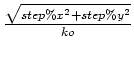$\frac{\sqrt{step\%x^2+step\%y^2}}{ko}$ . Suppose the error in the square root result $sqrt\_res$ is $E_{sqrt}$ , and the error in variable

is $E_{ko}$ , assuming the division unit itself does not bring extra error, the error in the division result is given by $E_{sqrt} \cdot \frac{sqrt\_res}{ko} + E_{ko} \cdot \frac{sqrt\_res}{ko^2}$ . As

holds a dynamic range from

, and $sqrt\_res$ has a maximum value of

(variables step%x and step%y have similar ranges), in the worst case, the error from $sqrt\_res$ can be magnified by 70 times, and the error from

magnified by approximately 9000 times. The values of $step\%x$ , $step\%y$ and

come from the software program as input values to the hardware circuit.

To solve this problem, we perform shifts at the input side to keep the three values $step\%x$ , $step\%y$ and

in a similar range. For

and the larger value between $step\%x$ and $step\%y$ , we perform the shifts so that the leading one of them is just right to the fractional point (in the form of $0.1\cdots$ ); for the smaller value between $step\%x$ and $step\%y$ , we assure it is shifted by the same distance as the larger value. The shifting distance difference between the

and $step\%x$ is recorded, so that after the division, the result can be shifted back into the correct scale. In this way, the $sqrt\_res$ has a range of

and

has a range of

. Thus the division only magnifies the errors by an order of 3 to 6. Meanwhile, as the three variables $step\%x$ , $step\%y$ and

are originally in single precision floating-point representation in software, when we pass their values after shifts, a large part of the information stored in the mantissa part can be preserved. Thus, a better accuracy is achieved through the shifting mechanism for fixed-point designs.

Fig. 5 shows experimental results about the accuracy of the table index calculation when using shifting or not using shifting, with different uniform bitwidths. The possible range of the table index result is from 1 to 2001. As it is the index for tables with smooth sequential values, an error within five indices is generally acceptable. We assume that the table index results calculated with double precision floating-point representation are accurate enough and use them as the true values for error processing. When the uniform bit-width of the design changes from 10 to 20, designs using the shifting mechanism show a stable maximum error of 3 and an average error around 0.11. On the other hand, the maximum error of designs without shifting vary from 2000 to 75, and the average errors vary from approximately 148 to 0.5. These results show that the shifting mechanism provides much better accuracy for the part of the table index calculation in fixed-point designs.

The other issue to consider is the representation of `wfld' data variables. As shown in the table above, both the real and imaginary parts of `wfld' data have a wide range from $10^{-14}$ to

. Generally, fixed-point numbers are not suitable for representing such wide ranges. However, in this seismic application, the `wfld' data is used to store the processed image information. It is more important to preserve the pattern information shown in the data values rather the data values themselves. Thus, by omitting the small values, and using the limited bit-width to store the information contained in large values, fixed-point representations still have a better chance to achieve accurate image in the final step. In our design, for convenience of bit-width exploration, we scale down all the `wfld' data values by a ratio of $2^{-22}$ so that they fall into the range of [0, 1).