Description of the Synthetic Data

The velocity model used to generate the synthetic data is shown in Figure 5. The water bottom is deep, flat in the inline direction and dipping at 15 degrees in the crossline direction. The only reflector is a plane dipping 3 degrees in the inline direction and 15 degrees in the crossline direction.

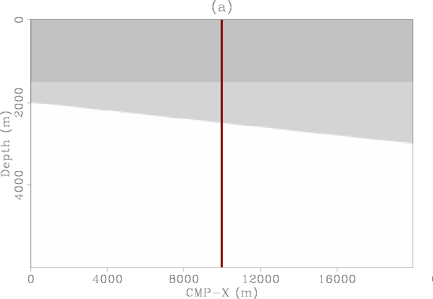
model-vel
Figure 5. 3-D velocity model. Panel (a) is the inline section taken at CMP-X=2000 m and panel (b) is the crossline section taken at CMP-Y=10000 m. The water-bottom dips in the crossline direction only. The reflector dips gently (3 deg) in the inline direction as well.

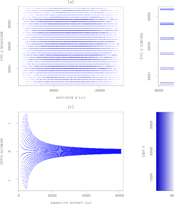
The acquisition geometry consists of 10 receiver lines, each with 240 receivers spaced 25 m, with the first receiver at an inline offset of 100 m from the source. The maximum inline offset is therefore 6075 m. The receiver line separation is 100 m and the source is flip-flop with the two sources separated 50 m in the crossline direction and centered between the two middle streamers. There are a total of 6 sail lines with each sail line separated from the next by a crossline distance of 450 m. With this arrangement, the crossline fold is just one and the fold in the inline direction is 60. Figure 6 shows a schematic of two adjacent sail lines illustrating that there is no overlap between the CMP coverage of each sail line. Figure 7 shows the receiver map, the source map, the azimuth-offset distribution and the fold map, all typical of a dual source acquisition.

sketch2 Figure 6. Schematic of fold coverage of two adjacent sail lines.

attributes
Figure 7. Top left: receiver map. Top right: source map. Bottom left: azimuth-offset distribution. Bottom right: fold map.

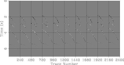
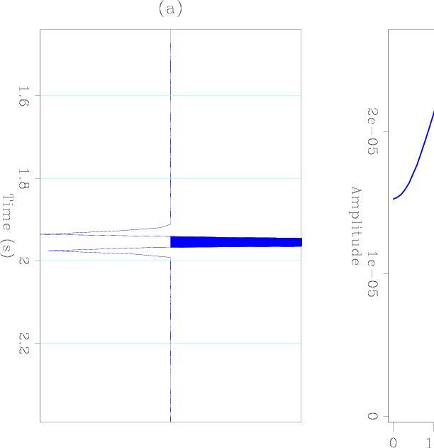
Figure 8 shows a typical common source record with the 10 receiver lines plotted side-by-side. There are four reflections: the water-bottom primary, the deeper reflector primary, the water-bottom multiple and the peg-leg multiple between the water-bottom and the deeper reflection. Notice the change in polarity of the multiples compared to the primaries. Figure 9 shows a close up of the wavelet and the wavelet spectrum which shows that the wavelet has a DC component.

shot
Figure 8. A typical ``shot'' gather showing the 10 receiver lines. Notice the polarity inversion of the multiples.

spectrum
Figure 9. Close up of the seismic wavelet (a) and its frequency spectrum (b). Notice the uncharacteristic presence of low frequencies usually absent in field data.