Data Subset for S-R Migration

The original dataset contains 6,764,207 traces (about 44 GB). Choosing a small, meaningful, ``complete'' five-dimensional subset of data for source-receiver migration is not trivial, because the acquisition geometry makes the offset distribution of adjacent CMPs different in both inline and crossline directions. This is illustrated in Figure 10 which shows the offset distribution inline for a few adjacent CMPs. The offset distribution repeats only every fourth CMP. Although not shown, the situation in the crossline direction is worse. There are 20 different crossline offsets (from -475 to 475 m), but for any CMP line taken at a fixed crossline position, all traces correspond to the same crossline offset.

The input to the source-receiver migration algorithm is a regular 5-D cube $D(t,\mathbf{m},\mathbf{h})$, where $\mathbf{m}$ is the vector of surface position, $\mathbf{h}$ is the vector of surface offsets and $t$ is the traveltime. In order to create such a cube, even for a small dataset, a large number of null traces need to be inserted. For example, for a 4 by 4 km square of full-fold CMP data, we have: 51200 CMPs (at 12.5 by 25 m bin) each with 240 inline offsets (100 to 6075 m at 25 m sampling) and 20 crossline offsets (-475 to 475 m at 25 m sampling) for a total of 440 million traces. Since each trace has 1751 samples (7 seconds at 4 ms sampling interval), this means a dataset of almost 800 GB.

sketch3
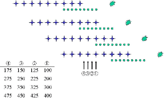
Figure 10. Schematic showing the unequal inline offset distribution of adjacent inline CMPs. The stars represent the receivers and the small circles represent the CMP positions. The table on the bottom left lists the inline offset distribution of a few traces corresponding to four arbitrary adjacent CMPs numbered 1 to 4 as indicated by the arrows. Notice that the adjacent CMPs have different inline offset distribution.

In order to make a more manageable dataset, further data reduction is necessary. Here I am particularly interested in the effect of crossline dip in the moveout of the multiples after migration, therefore I chose to subsample the data in the inline coordinates only. I subsampled the inline CMP axis such that every other CMP was discarded. This has the advantage of not only halving the number of CMPs but also halving the number of inline offsets as can be seen in Figure 10 since now the inline offset interval is 50 m rather than 25 m. I also subsampled the time axis to 16 ms, which required that the data be filtered to a maximum frequency of 32 Hz. The original wavelet had frequencies up to about 60 Hz as illustrated in Figure 9. High-cut filtering is acceptable in this case because vertical resolution is not critical for my purposes. I also limited the inline offsets to 4000 m which sacrifices the steeper flanks of the moveout of the multiples as shown in Figure 8. With these reductions, the dataset size becomes about 70 GB after some padding in all spatial directions to avoid or at least lessen migration artifacts.

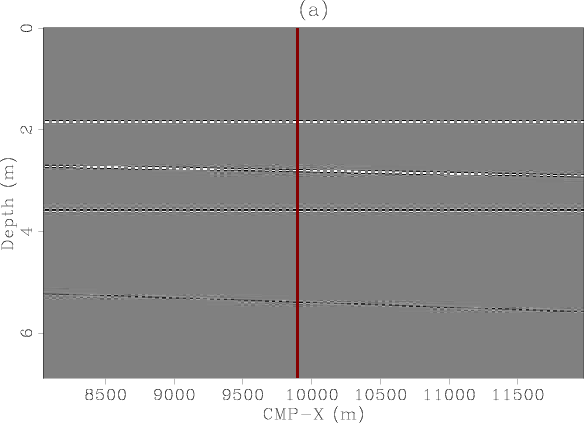
Figure 11 shows a near offset cube of the five-dimensional selected dataset. Notice that there are only six crossline CMPs for a given inline CMP location, corresponding to the six sail lines, and there is no data redundancy in the crossline direction. Similarly, only every other inline CMP position has a trace with a given crossline CMP location because of the dual shot geometry.

zoff1
Figure 11. Near offset cube (100 m offset inline and -25 m offset crossline). Panel (a) is the inline section at CMP-Y=1712.5 m while panel (b) is the crossline section at CMP-X=9925 m.

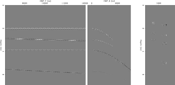
Panel (a) of Figure 12 shows the inline distribution of offsets for an inline CMP section taken at crossline CMP position 2212.5 and crossline offset of -12.5 m. Here again, note the on-off pattern of the offset distribution due to the dual shot source as indicated in the sketch in Figure 10. Similarly, panel (b) of Figure 12 shows the distribution of crossline offsets for a CMP section in the crossline direction taken at inline CMP location 8400 and inline offset of 100 m.

inline-xline
Figure 12. 3D data. Panel (a) is the inline section taken at 100 m inline offset, -25 m crossline offset and CMP-Y=-12.5 m. Panel (b) is the inline offset gather at CMP-X=8550 m, CMP-Y=-12.5 m and -25 m crossline offset. Panel (c) is the crossline section at CMP-X=8400 m, 100 m inline offset and 25 m crossline offset. Panel (d) is the crossline offset gather at CMP-X=8400 m, CMP-Y=1837.5 m and 100 m inline offset. Notice the data sparsity, especially in the crossline direction.