First Order Multiples - Analytics

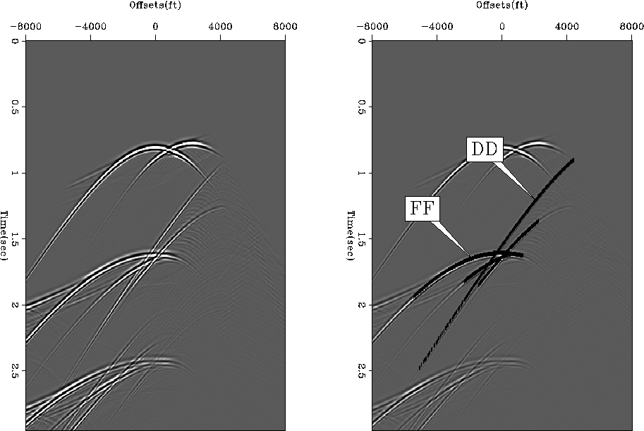
To identify different multiples and to understand their behavior, I analytically modeled the ray paths for all possible first-order multiple events for the given synthetic model. For simplicity of referencing to these events I use the nomenclature given in Table 1.

Table 1. Nomenclature for different first order multiples.

Type Ray-path Name

1 Both the bounces on the flat part FF

2 First bounce on the flat part and second on the dipping FD

3 First bounce on the dipping part and second on the flat DF

4 Both the bounces on the dipping part DD

 

shot5000
Figure 3 (a) A shot record corresponding to a shot located at a surface location of 5000. (b) Shot record with first order multiples modeled analytically overlaid on them

Equations 4 and 5 give the travel time and offset as a function of $\theta$ (take-off angle) for the event FF,  

$$t(\theta)=\frac{4d}{V \cos\theta},$$ (4)

 

$$h(\theta)=4 d \tan\theta .$$ (5)

In the equations above, d is the depth of the flat reflector, V is the velocity, and h and t are offset and travel time respectively. There are different conditions and constraints on the value of $\theta$ depending on the shot location, which determines the range of take-off angles where these events take place and get recorded. Equations 6 and 7 give the expressions for travel time and offsets for the event FD.

$$\begin{eqnarray} t(\theta)=\frac{1}{V}.\{\frac{2d}{\cos \theta} + \frac{(x_d + \... ...d + \frac{d}{\tan \alpha} - x_s - 2 d \tan \theta] + 2d\tan \theta\end{eqnarray}$$ (6) (7)

In these equations, x_d is the horizontal location where the dipping reflector meets the flat layer, x_s is the source location and $\alpha$ is the dip of the dipping reflector. There are two other possibilities for the first-order multiples: DF and DD. Travel time and offsets are given in equations 8 and 9 for the first category and equations 10 and 11 for the second category.

$$\begin{eqnarray} t(\theta) = \frac{1}{V}\{(x_d+\frac{d}{\tan \alpha} - x_s)\frac... ...{\cos(2 \alpha - \theta)}] + \frac{2d}{\cos (2 \alpha - \theta)}\}\end{eqnarray}$$ (8)

$$\begin{eqnarray} h(\theta) = (x_d + \frac{d}{\tan \alpha} - x_s).\frac{\sin \alp... ...os \theta \tan(2 \alpha - \theta)) - 2 d \tan (2 \alpha - \theta\}\end{eqnarray}$$ (9)

$$\begin{eqnarray} t(\theta) &=& \frac{1}{V}.[x_d + \frac{d}{\tan \alpha} - x_s].\... ...a - \theta)}.\frac{\cos(\theta- \alpha)}{\cos(3 \alpha - \theta)}]\end{eqnarray}$$ (10)

$$\begin{eqnarray} h(\theta) &=& [x_d + \frac{d}{\tan \alpha} - x_s].\frac{\sin \a... ...a - \theta)}.\{\tan(2\alpha - \theta) + \tan(4 \alpha - \theta)\}]\end{eqnarray}$$ (11)

Once again, all the above equations are functions of the parameter $\theta$ and are valid only for a range of $\theta$ values corresponding to angles at which the event actually takes place. On Figure (b) are overlaid the first-order multiple events modeled using the above equations.