| d4Sz4+d3Sz3+d2Sz2+d1Sz+d0=0, | (1) |

![[*]](http://sepwww.stanford.edu/latex2html/cross_ref_motif.gif) shows how the dispersion relation
looks, given the anisotropy parameters
shows how the dispersion relation
looks, given the anisotropy parameters Conventional implicit finite-difference methods are designed by truncating the Taylor series of the dispersion relation. The dispersion relation for TTI media is so complex that it is difficult to derive an analytical Taylor series used for an implicit finite-difference scheme.
Generally, the Padé approximation suggests that
if the function ![]() , then Sz(Sx) can be approximated by a rational function
Rn,m(Sx):
, then Sz(Sx) can be approximated by a rational function
Rn,m(Sx):
| (2) |
![]()
![]()
Sz is an even function of Sx for isotropic and VTI media. In contrast, Sz is not an symmetric function of Sx for TTI media. It's well known that an general function can be decomposed into an even function and an odd function. We approximate the even part of the dispersion with the even rational functions, such as Sx2, Sx4 and approximate the odd part with odd rational functions, such as Sx,Sx3.
 |
Considering the stability of the finite-difference scheme, I approximate the dispersion relation of TTI media with rational functions as follows:
| |
(3) |
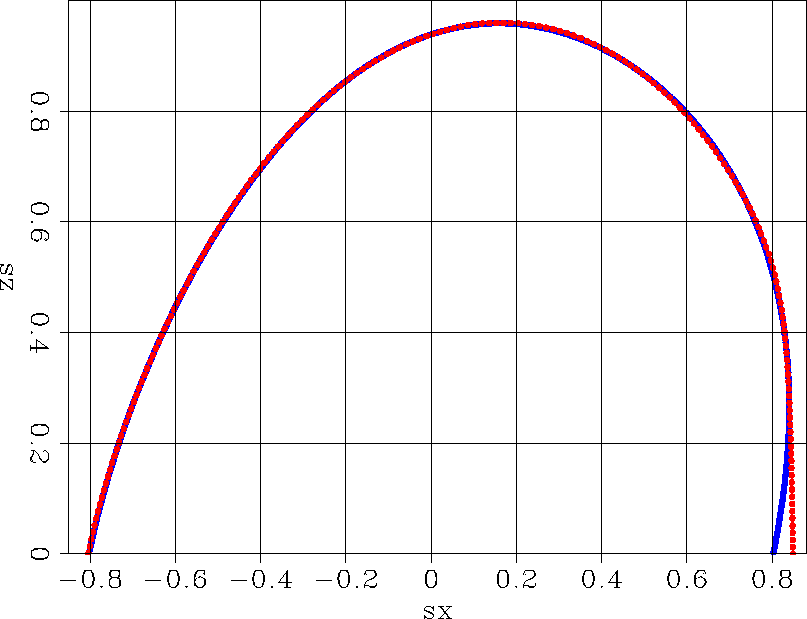
![[*]](http://sepwww.stanford.edu/latex2html/cross_ref_motif.gif) compares the true dispersion relation with the approximate dispersion relation.
The solid line is the true dispersion relation (equation 1) and the dashed line is the approximate dispersion relation for the finite-difference
scheme ( equation 3). The dispersion relation for the finite-difference scheme is very close to the true one for the negative
Sx. When the phase-angle is close to
compares the true dispersion relation with the approximate dispersion relation.
The solid line is the true dispersion relation (equation 1) and the dashed line is the approximate dispersion relation for the finite-difference
scheme ( equation 3). The dispersion relation for the finite-difference scheme is very close to the true one for the negative
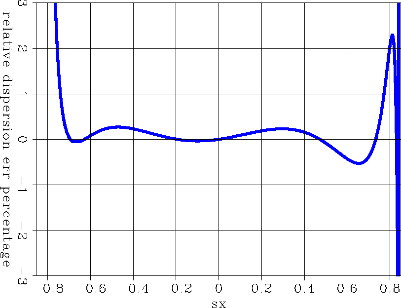
Sx. When the phase-angle is close to ![[*]](http://sepwww.stanford.edu/latex2html/cross_ref_motif.gif) shows the relative dispersion error defined as follows:
shows the relative dispersion error defined as follows:
| (4) |
 |
For a laterally varying medium, the anisotropy parameters vary laterally. As a consequence, the coefficients for
the finite-difference scheme vary laterally.
It is too expensive to estimate these coefficients for each discrete grid during the wavefield extrapolation.
After estimating the minimum and maximum value of the anisotropy parameters and the tilting angle,
I compute the coefficients for the anisotropy parameters and the tilting angle in these ranges and store them in a table before the migration.
During the wavefield extrapolation, given the anisotropy parameters ![]() ,
, ![]() , and the tilting angle
, and the tilting angle ![]() ,
I search the coefficients in the table and put them into the finite-difference scheme.
Given the coefficients found from the table, the finite difference algorithm in TTI media is the same as the isotropic media.
The table of coefficients is small, and the computation cost for table-searching is trivial compared to
that of solving the finite-difference equation. Therefore, the cost of the optimized implicit finite-difference for TTI media
is similar to that of the conventional finite-difference methods for isotropic media.
,
I search the coefficients in the table and put them into the finite-difference scheme.
Given the coefficients found from the table, the finite difference algorithm in TTI media is the same as the isotropic media.
The table of coefficients is small, and the computation cost for table-searching is trivial compared to
that of solving the finite-difference equation. Therefore, the cost of the optimized implicit finite-difference for TTI media
is similar to that of the conventional finite-difference methods for isotropic media.
 |